In the first blog post on the response spectrum, the idea of how such a spectrum is created was discussed. However, why this is created and how to use this for any engineering purpose, was not discussed. In this blog post we will have a closer look at how to utilize such a spectrum for a (almost) realistic loading case. So, as Matt Trakker would have said: Spectrum on!
Where to start?
Ok, let us assume that we have been given the response spectrum that was created in the last blog post on this subject, how do we use it for engineering good? Well, one way is to try to plug the information into a finite element code and see what input it needed. As an example, let’s have a look at the input card related to response spectrum for Ls-Dyna:
It appears that the code is very eager to compute the natural modes, since a lot on the input parameters are related to that. The first 4 parameters are related to the natural modes, so this must be of some importance. However, I do not know how yet. There also exist some parameters that are related to the actual spectrum and in what direction is used and at what location on the structure. That this information is needed seems rather obvious. And finally, there is some information on how to combine the different modes. Hmm, don't really know what that is.
Ok. Now we have some idea of what is needed, but currently I do not really know why this is needed. So, let's grab a pen and paper and see if we can make some sense out of this.
Back to (engineering) school
At least for me, when trying to learn new things, a good way to start is to investigate a simple example. In this blog post, this simple example will be a (not so realistic) five story house as shown in the figure below.
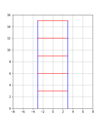
In the calculations, it is assumes that the “floor” is rigid compared to the “columns” and also that the mass of the columns are small compared to the mass of the floor. The calculations will be done without the influence of damping.
First, let's have a look at the natural modes for the five story building. Below two animations can be seen. Both show the “house” after some initial perturbation of the floors has been released.
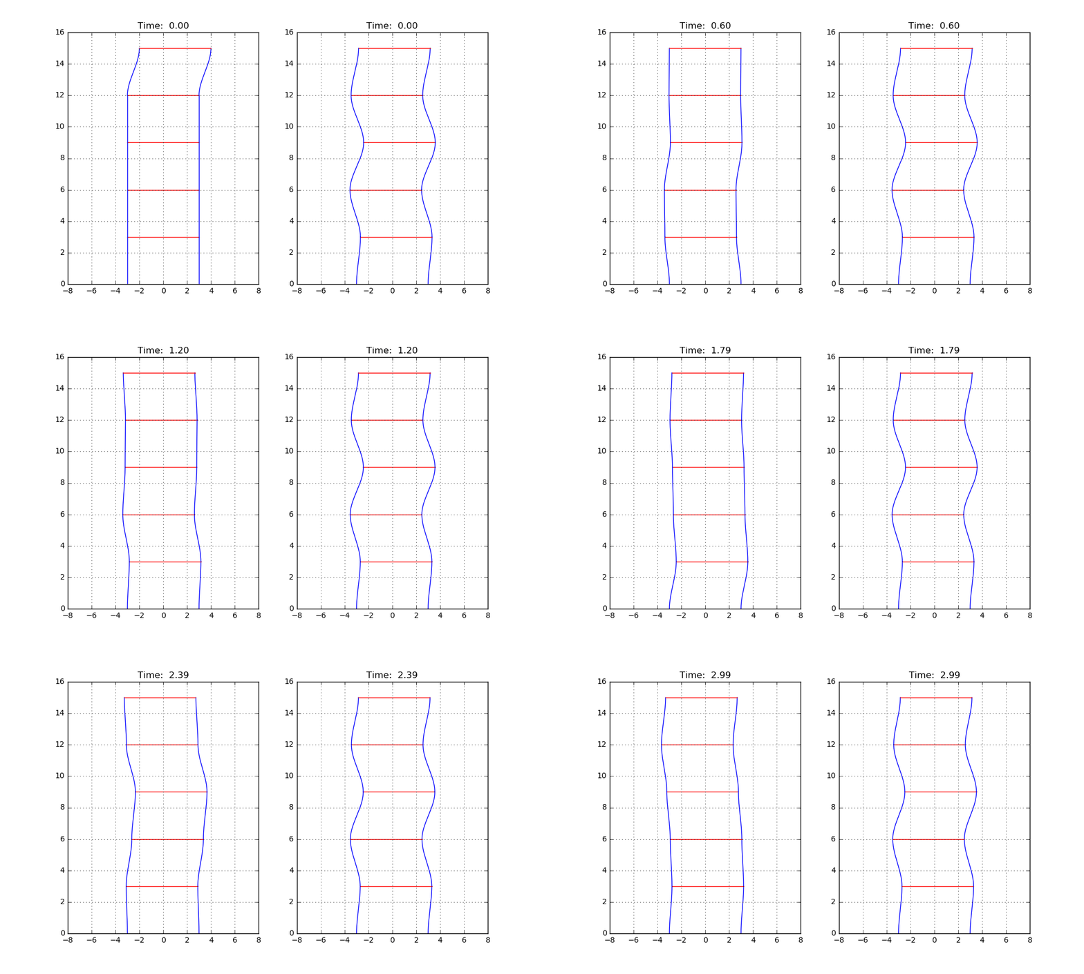
These perturbations are different for the left and right example. In the example to the left, deformation of the floors almost seem random. However for the example to the right, a uniform repetitive deformation shape can be seen, indicating a natural mode
One way to find these modes would be to test a lot of examples as the one above and se what shapes that turns out to be natural modes, but this would be a real time consuming task (and really boring). So let's try some math instead.
Let's start by investigate the following system and as mentioned earlier, this system is undamped. Since there is no external forces acting on the system, this is called system under free vibrations.
Consider that the shape in the animation to the right above would look something like this
Alright, this one I recognize from linear algebra. This is an eigenvalue problem that I know how to solve.
The eigenvalue here are the
import numpy as np
import scipy as sp
from scipy import linalg
import scipy.interpolate
import matplotlib.pyplot as plt

# Define mass and stiffness matrix:
m = 453.59237 * 100.0
k = 31.54 * 175126.7909209900

K = k * sp.matrix([[ 2.0, -1.0,  0.0,  0.0 , 0.0],
                   [-1.0,  2.0, -1.0,  0.0 , 0.0],
                   [0.0,  -1.0,  2.0, -1.0,  0.0],
                   [0.0,   0.0, -1.0,  2.0, -1.0],
                   [0.0,   0.0,  0.0,  -1.0, 1.0]] )
M = m * np.eye(5,5)

# Solve generalized eigen value problem to find natural modes and frequencys:
eig,eigv = linalg.eig(K,M)
Ok! Now we have figured out what a natural mode is, but not why it is useful in this context. Therefore, let's try something different. Lets us define the displacement by using the natural modes as basis according to:
Here
The
OK, so far it is no obvious that describing the displacements using the natural modes will give any great advantage.
So let’s go a little crazy! Why not consider a special type of external loading (that is quite common).
This special case is where
This seems somewhat strange, but can be interpreted as inertia forces associated with the different modes.
The
Now, let's try to insert the this expansion of the external forces into the equation of motion above. By using the orthogonal properties of the natural modes gives:
Where
Not bad at all! Now we are back to a problem that looks a whole lot like the single degree of freedom system that we solved in the first blog post on this subject. Let's arrange the expression somewhat more and it will look so even more:
Here we just have divided the equation by
Here the “n” indicated that this forces are computed for the n:th mode. Plugging the definition of displacement for the n:th mode and using the expression for the eigenvalue problem earlier in the post gives:
Alright! This final expression makes a pretty cool interpretation possible. The equivalent static forces may be interpreted as the static forces multiplied by some factor that is related to the dynamics of the system. An even cooler this is that this is possible to generalize according to:
OK, here
That was quite a lot of equations… Lets see what kind of magic this can work for the five story building exposed to earthquake situation.
Boom shake the room
So, let’s try to summarize a strategy on how to solve this five story building exposed to the earthquake load.
Given that the external force acting on the house
- Compute the natural modes
- Compute the modal participation factor
- Compute
- Compute
- Compute the dynamic response by
This does not seem to be that difficult to implement, why not give it a go for the five story building.
In this case, it can be shown that
Dt = 0.02
m1 = 1.0
psi = 0.05

s = np.array([1.0,1.0,1.0,1.0,1.0])

# Get V_base_stat
V_b_st = []

# Compute fall all natural modes
for i in range(len(eig)):

    Mi = np.dot(eigv[i],np.dot(M,eigv[i]))
    Li = np.dot(eigv[i],np.dot(M,s))

    # Compute modal participation factor
    hi = Li/Mi

    # Compute D
    k = eig.real[i]
    t_vec,u_vec,u_dot_vec = GetMaxResponce(k,m1,psi,Dt,Data_acc)

    # Compute base force
    sn = eigv[i]*hi*m
    V_b_st.append( np.sum(sn)*np.array(u_vec)*eig[i] )
That was not too much code but still makes great things! Let’s plot the resulting shear force at ground level associated to the different modes. This can be seen below.
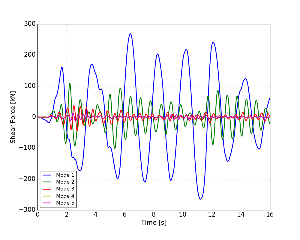
When looking at the figure, a few things are worth mentioning. The first mode looks to have the greatest impact on the shear force. Also, the maximum shear force occurs at different points in time for the different modes.Let’s have a look at the total shear force:
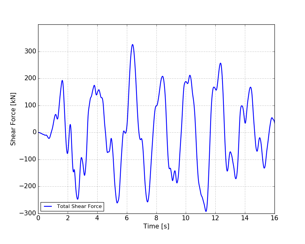
Nice! The maximum total shear force is approximately 325 kN.
OK, but how do I use the freaking spectrum?
That is a fair question. So far I have only ranted about eigenvalues, orthogonality or other things, but where does the spectrum (as shown below) fit into the picture?
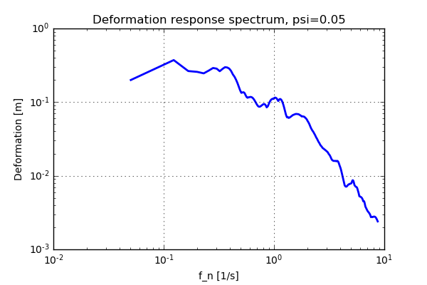
The method presented above will give the time history of the response
Can the peak response be determined directly from the response spectrum for the ground motion without computing the entire time history?
For a system of single degree, this would be possible but for a system of multiple degree (as the five story building) the answer would be a qualified “yes”. As seen above, the time when the maximum response occurs differs for the different modes and by simply adding up the absolute values (ABSSUM method) will probably be a little to conservative. Another method that is used is the “square root of sum squared” (SRSS method). As mentioned, these are approximations and will in general not give the same result as evaluating the time history. These are summarized below:
This does not look to be too complicated. Also, when using the response spectrum to
compute the peak loading condition all that has to be replaced is the computation of
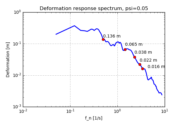
Now all that's left to do is just to perform the calculations. Below a table is shown where the maximum total shear force on ground level can be seen for the different computation methods.
| Method | Max shear force |
|---|---|
| ABSSUM | 437 kN |
| SRSS | 294 kN |
| Time history | 325 kN |
Time to conclude
First of all, this blog post was about twice the size as I had planned at the beginning. But once you get started it is kind of hard to stop… I found the mathematics to be really cool, especially the advantages that the decomposition using the natural modes give.
Hope you enjoyed this post and as usual, if you have questions or comments please contact us.
Reference
A.K. Chopra (2000). Dynamics of structures (Second edition). Prentice Hall