For those of you who are interested in or/and working with finite element simulations, chances are that you have seen or ever performed some kind of structural optimization. Most of today's commercial codes have this feature and some really impressive work can be done by just pushing some buttons in the pre-processor. Out comes an optimized structure just like magic. But how much “magic” is actually needed to do this? This is the subject for this blog post.
So what is optimization?
We should probably start with just investigating the words “structural optimization”. In the great book “Introduction to structural optimization” by Christensen and Klarbring, you can find:
- Structure: Any assembly of materials with the intent to sustain load
- Optimization: Making things great (the best they can be)
So, structural optimization is “making an assembly of material sustain load in the best way”. Of course, what is best has to be defined and usually there are some constraints that have to be fulfilled. In general, one speaks of three different types of structural optimization:
- Sizing Optimization: This is where some structural thickness is optimized. Could be the cross section area of a beam or bar.
- Shape Optimization: Where the form or contour is optimized
- Topology Optimization: The pinnacle of optimization (if you ask me). This is the cool optimization where a massive piece of material is turned into beautiful structures to sustain the loads.
In this blog post the first kind of optimization will be investigated, but my intention is to come back with a go at the third one as well. So let’s start.
Let's go to the bar(s)
As usual, when learning new things, a simple but illustrative example is useful to study. In this case we will use a (probably not so realistic) structure containing a number of steel bars, see the picture below:
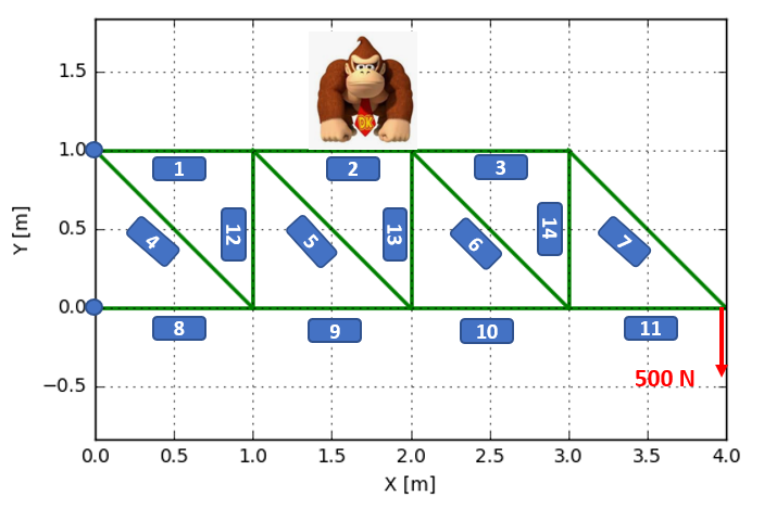
The structure is subjected to a load, in this case a point load at the end of the structure (monkey is excluded). There are also some points where the structure is attached to a wall (marked by blue dots). The numbers that are found in the picture are the element numbers, and will be used later on.
Since I am a person that does not like to spend money when I don't have to, the total mass of the structure can not be heavier than 1000 kg. And those kilos have to do the best job possible to sustain the load at the tip. The request of the structure not to be heavier than 1000 kg can here be seen as some sort of constraint. If we define the cross section area of a bar as \( x_i \) and the length of the bar as \(l_i \) the following constraint can be formulated as:
\[ g_1 = \sum_{i=1}^n l_ix_i - V_{max} \leq 0 \]Note that \(A_{min} \le x_i \le A_{max} \). It was not that difficult to formulate the request on weight on some mathematical thermes, but what about the request that the structure should do the best job possible to sustain the load? Well, there exists a number of possibilities, but here we will try to minimize the compliance defined as:
\[ g_0 = {\bf F}^T{\bf u} \]Sweet! Now we more or less have defined an optimization problem, and these kinds of problems have been studied in great detail by a lot of smart guys. From here on, \(g_0\) will be called the “objective function” and \(g_1\) will be call constraint
Find a plan
Much effort has been but into optimize (minimize) convex functions subjected to inequality constraints. Now this sounds very interesting to use, but to be honest, I do not know if the function that I would like to minimize (the compliance) is convex or not? I could of course take the time to investigate if that is the case, or I could simply use some sort of approximation that I for sure know is convex. The latter option sounds like less work, so let's go for that. By doing this type of approximation, the following strategy solve the problem can be constructed:
- Start with an initial design where the cross section areas can be collected in the vector \(x^k\) where k=0
- Calculate the displacements for the current design by solving a finite finite element problem \(K(x^k)u(x^k) = F(x^k) \)
- For the current design \(x^k\), calculate the objective function, the constraint function and their gradients.
- Formulate an explicit, convex approximation to the optimization problem at \(x^k\)
- Solve the approximation by a nonlinear optimization algorithm to find the new design \(x^{k+1}\)
- put k = k+1 and return to step 2 unless some smart stopping criterion is satisfied.
OK, now we have a plan. Let's spend some time on point 2, even if this is not the topic for this blog post. Here you can use your favorite solver, but here I have used “Calfem for python” which can be downloaded here. The structure in the figure above can be defined as:
rho = 7800
Amax = 0.1
Amin = 1.0e-9
ndof = 18
nelm = 14
Vmax = 1000.0/rho
dofs = np.array([[1,2],[3,4],[5,6],[7,8],[9,10],[11,12],[13,14],[15,16],[17,18]])
Coord=np.array([[0.0,1.0],
                [1.0,1.0],
                [2.0,1.0],
                [3.0,1.0],
                [0.0,0.0],
                [1.0,0.0],
                [2.0,0.0],
                [3.0,0.0],
                [4.0,0.0]])
Edof = np.array([[1,2,3,4],
                 [3,4,5,6],
                 [5,6,7,8],
                 [1,2,11,12],
                 [3,4,13,14],
                 [5,6,15,16],
                 [7,8,17,18],
                 [9,10,11,12],
                 [11,12,13,14],
                 [13,14,15,16],
                 [15,16,17,18],
                 [3,4,11,12],
                 [5,6,13,14],
                 [7,8,15,16]])

bc = np.array([1,2,9,10])


ex,ey = co.coordxtr(Edof,Coord,dofs)

A = np.ones(nelm)*0.1*0.0819
E = 210e9
F = 500
For those not familiar with CalFem or the finite element method, this looks somewhat weird. The documentation is found on this link.
One the structure is defined, there is not much code needed to get the displacements.
# Create empty stiffnes matrix
K = np.mat(np.zeros((ndof,ndof)))
f = np.mat(np.zeros((ndof,1)))
f[-1] = -F

# Set up and solve problem
for i in range(nelm):
    ke = co.bar2e(ex[i],ey[i],[E,A[i]])
    K =  co.assem(Edof[i],K,ke)

(a,r) = co.solveq(K,f,bc)
Ed = co.extractEldisp(Edof,a)
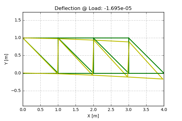
Note that initial cross section areas are selected so that the total mass of the system is 1000 kg. Also, the cross section areas are allowed to vary between 0.1 and 1e-9. Below the defored shape of the structure can be seen (scaled) and the displacement at the loading point is also written out. It is expected that this displacement will decrease for an optimal design.
Now let's focus on point 3, 4 and 5. Lets start by looking at two common approximations: The Sequential Linear Programming (SLP) and Sequential Quadratic programming (SQP). The SQP approximation can be seen below:
\[g_0^{SQP} = g_0({\bf x}^k) + \nabla g_0({\bf x}^k) ({\bf x}-{\bf x}^k)+0.5({\bf x}-{\bf x}^k)^T{\bf H}({\bf x}-{\bf x}^k) \]
Here the objective function is approximated by first and second order derivatives (\( {\bf H} \) is here the Hessian). To get the SLP approximation, simply remove the second order term. These two approaches are widely used to solve general nonlinear optimization problems, and this may sound like a good thing, right? But perhaps there is an approach that is more tailored to our need, i.e. that fits the properties that this structural optimization problem has?
Well, one such approach is the Convex Linearization (CONLIN). One can conclude that the stress and displacements are connected to the cross section area in a reciprocal way, i.e. like \(1/x_i\) where \(x_i\) is the cross section area. This holds when the system is statically determined, but it seems to be reasonable to use this even when the system is not statically determined. However, it would be a bad idea to linearize every type of function with respect to \(1/x_i\). So what if some variables could be linearized in \(x_i\) and some in \(1/x_i\)? This is exactly what is done in the CONLIN approximation, and is written as:
\[ g_0^C = g_0({\bf x}^k) + \sum_{j \in \Omega_+ } g_{0j}^{L,k}({\bf x}) + \sum_{j \in \Omega_- } g_{0j}^{R,k}({\bf x})\]
Humm, does not look that simple. A lot of crazy letters and domains. But here the \( g_{0j}^{L,k} \) and \( g_{0j}^{R,k} \) are defined as:
\[ g_{0j}^{L,k} = \nabla_j g_0({\bf x}^k) (x_j-x^k) \]
\[ g_{0j}^{R,k} = \nabla_j g_0({\bf x}^k) x_j^k (x_j-x_j^k)/ x_j \]
Futhermore, the domains \( \Omega_+ \) is where the gradient is possitive and \( \Omega_- \) is where the gradient is negative
Alright! Now we have found a way to approximate our problem, but how do we solve it? Thinking back to some lecture in mathematics way to long ago, I remember that when solving these kinds of problems, the Duality formulation makes life somewhat easier. This is created by introducing the Lagrangian function such as:
\[ L({\bf x},\lambda) = g_0 + \lambda g_1 \]
The introduced parameter \( \lambda \) is known as a Lagrangian multiplyer. Note that if more than one constrain function was present, there would exist multiple Lagranginan multipliers.
where the dual objective function is defined as
\[ max \, \psi(\lambda) \]
where
\[ \psi(\lambda) = min \, L({\bf x},\lambda) ) \]
This also looks somewhat difficult, but lets have a look at the two problems. First we find the x that minimizes \( L({\bf x},\lambda) \). Once \(x_i\) has been found (expressed in \( \lambda \)), find the \( \lambda \) that maximize the dual objective function.
Let's optimize
We have already looked into the Finite Element solver so the displacements for the initial design we already know. Now let's look at the approximation for this given problem. Following the definition above, the objective function can be approximated as:
\[ g_0^C = {\bf F}^T {\bf u}({\bf x}^k) - \sum_{j=1}^{n} {\bf u}_j^T({\bf x}^k) {\bf k}_j^0 {\bf u}_j ({\bf x}^k) (x_j^k-(x_j^k)^2/x_j) \]
Here use has been made of that the derivative of compliance is always negative. Moreover, since the constraints already are linear in \(x_i\), there is no need to introduce any approximation. The local stiffness matrix for the j:e element is related to \({\bf k}^0 \) as
\[ {\bf k}_j = x_j{\bf k}_j^0\]
The Lagrangina for this problem can be defined as:
\[ L({\bf x},\lambda) = {\bf F}^T {\bf u}({\bf x}^k) - \sum_{j=1}^{n} {\bf u}_j^T({\bf x}^k) {\bf k}_j^0 {\bf u}_j ({\bf x}^k) (x_j^k-(x_j^k)^2/x_j) +\lambda (\sum_{i=1}^n l_ix_i - V_{max}) \]
Now let's start by assuming that the minimum is obtained for the \(x_j\) value for which the partial derivative of \(L\) with respect to \(x_j\) is zero:
\[ \nabla_j L({\bf x},\lambda) = -{\bf u}_j^T({\bf x}^k) {\bf k}_j^0 {\bf u}_j(x_j^k)^2/x_j^2 + \lambda l_j = 0\]
wich gives:
\[ x_j = \sqrt{{\bf u}_j^T({\bf x}^k) {\bf k}_j^0 {\bf u}_j(x_j^k)^2/(\lambda l_j) } \]
if now \(x_j\) is smaller than \(A_{min}\), let's simply put the \(x_j\) value to \(A_{min}\). If \(x_j\) is larger than \(A_{max}\) let's put the value to \(A_{max}\). All that now is left to do is to solve the scalar dual problem. Lets create a function that for a given lambda computes the value of the dual objective function.
def GetDual(lam,ex,ey,E,A,f,a,nelm,Ed,Amax,Amin,Vmax):
    Ck = np.asscalar(f.T*a)
    A1 = []
    A2 = []
    for i in range(nelm):
        ke = co.bar2e(ex[i],ey[i],[E,1.0])
        ci = np.asscalar(np.mat(Ed[i].reshape(1,4)) * ke * np.mat(Ed[i].reshape(4,1)))
        li = np.sqrt(np.diff(ex[i])**2+np.diff(ey[i])**2)

        xi = np.sqrt(ci*A[i]**2/(li*lam))

        if xi > Amax:
            xi = Amax
        if xi < Amin:
            xi = Amin
        A1.append( ci*(A[i]-A[i]**2/xi) )
        A2.append( li*xi )

    # Construct dual function
    psi = -(Ck - np.sum(A1)+ ( np.sum(A2) - Vmax )*lam)

    return psi
When we have this function defined, some fancy build in functionality can be used to solve the scalar problem. Here the scipy.optimize function fmin is used. We will also need a function that for a given value of lambda, returns the new value of the cross section areas. This can be found below.
def GetAreas(lam,ex,ey,E,A,f,a,nelm,Ed,Amax,Amin,Vmax):
    # For a given value of lam, returns:
    # Areas    Vector containing bar areas
    # Ck       Current value of compiance
    # V        Current volume of structure
    Ck = np.asscalar(f.T*a)
    Areas = []
    Vol = []
    for i in range(nelm):
        ke = co.bar2e(ex[i],ey[i],[E,1.0])
        ci = np.asscalar(np.mat(Ed[i].reshape(1,4)) * ke * np.mat(Ed[i].reshape(4,1)))
        li = np.sqrt(np.diff(ex[i])**2+np.diff(ey[i])**2)

        xi = np.sqrt(ci*A[i]**2/(li*lam))
        xi = np.asscalar(xi)
        if xi > Amax:
            xi = Amax
        if xi < Amin:
            xi = Amin

        Areas.append(xi)
        Vol.append(xi*li)

    return Areas,Ck, np.sum(Vol)
Bar optimization - Take 1
That great! Now we have all that is needed to put the entire code together. It will not be much but it will be good! Behold:
# Create empty stiffnes matrix
f = np.mat(np.zeros((ndof,1)))
f[-1] = -F

for ii in range(4):
    K = np.mat(np.zeros((ndof,ndof)))
    # Set up and solve problem
    for i in range(nelm):
        ke = co.bar2e(ex[i],ey[i],[E,A[i]])
        K =  co.assem(Edof[i],K,ke)

    (a,r) = co.solveq(K,f,bc)
    Ed = co.extractEldisp(Edof,a)

    # Solve duality problem to find new lambda_star
    lam_star = fmin(GetDual,0.1,(ex,ey,E,A,f,a,nelm,Ed,Amax,Amin,Vmax))
    # Find new areas of bars
    Areas,Ck,Vol = GetAreas(lam_star,ex,ey,E,A,f,a,nelm,Ed,Amax,Amin,Vmax)
    A = Areas

# Get Normal forces in bars
En = []
for i in range(nelm):
    En.append( co.bar2s(ex[i],ey[i],[E,A[i]],Ed[i]) )
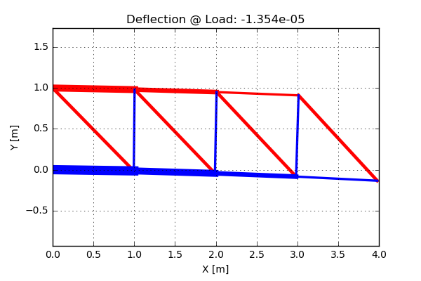
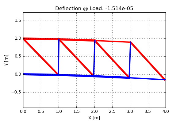
Here the number of iterations has been set to 4, which is enough for convergence. Lets now have a look at the cross section areas after the optimization. In the picture below the thickness of the bars are related to the cross section areas. In addition, the red bars are loaded in tension and the blue bars are loaded in compression. The deflection at the loading point is now smaller than for the original design, sweet!!
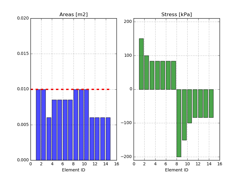
OK, now let's have a closer look at the cross section areas and the stresses in the different bars. From an intuition point of view, it would be expected for the stresses to have the same absolute value for all bars. If this is the case, all bars are "equally" used. Lets plot the cross section areas and the stresses for the different bars. The result can be seen below:
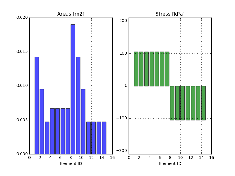
Nice! Looking at the stresses in the bars, this above described intuition looks to be true. Here the absolute value of the stresses are equal for all bars. An other thing to notice is that the largest cross section area is no were close to the \(A_{max} = 0.1\)
Bar optimization - Take 2
What if we now would pick a smaller \(A_{max}\), say 0.01. Looking that graph above, there are some bars that would be affected of such a condition. Furthermore, the assumption that all bars should have the same absolute value when it comes to the stresses, may not hold any more. For the bars that has reached the maximum value of the cross section area, it would be expected to have a higher stress that the ones that have not reached the maximum area. Let's simply change the \(A_{max}\) parameter and rerun the code. Results are shown below.
Bar optimization - Take 3
Let's investigate one final version of the same problem. Let's assume that someone added one bar to the system. The bar is marked in red in the figure below: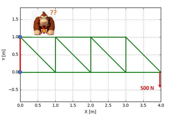 Dude, that some waste of good steel. The bar is attached to the two nodes that are connected to the wall, so this bar would do nothing more
that just add mass to the system. If the method is working, this bar should have a very small cross section area after the optimization.
So, let's try it out. All that has to be done is to add one extra row to the Edof matrix looking like [1,2,9,10]. After running the
optimization, it can be concluded that the area of the bar now is \(A_{min}\) and the rest of the results are the same as for the second
problem. Once more, the code looks to be doing the right thing!
Time to conclude
Ok, this was the first of two posts on the subject of structural optimization. In this post, the sizing problem was investigated. It is worth mentioning that there are even more options when it comes to choice of approximation, but for the purpose of this plot post, the CONLIN approximation looks to work fine.
Hope you enjoyed this post and as usual, if you have questions or comments please contact us.
Reference
P.W Christensen and A Klarbring. An introduction to structural optimization (2009). Springer