Structural Optimization - Part 2

In the first part on the subject of structural optimization, we started with an overview of different types of optimizations. In that post we had a deep dive in what is called sizing optimization, and a simple steel bar system was optimized when it comes to cross section areas of the bars. In this post we will have a closer look at the topology optimization. As the title of this post implies, what we want to accomplish is, starting from one massive piece of material, remove material that is not needed.

Let's create some holes

If you have read some of our old posts, you probably realized that including some simple but illustrative examples as a starting point to learn new things is our cup of tea. This post is no different. Below a L-shaped piece of steel that is loaded in one end and attached to the “roof” in the other end. At the end of this post we hope that somehow a lot of material has been removed from the structure and left is only the “good” material that makes the structure stiff.

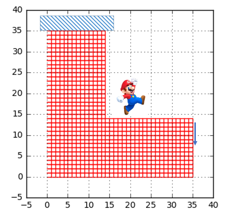
Let's start by looking at what we manage to accomplish in the first post on this subject. To recap we would like to minimize the compliance, defined by:

\[ g_0 = {\bf F}^T{\bf u} \]

and this is done under some constraints, here limiting the volume of the structure:

\[ g_1 = \sum_{i=1}^n l_ix_i - V_{max} \leq 0 \]

Recall that last time we investigated a steel bar structure and here the \(l_i \) represent the length of a bar and \( x_i \) is the cross section area. However, this does not sound to different what we would like to achieve, so let's do a slight reformulating of the constraint:

\[ g_1 = \sum_{i=1}^n \rho_iA_it_i - V_{max} \leq 0 \]

Here we have introduced some sort of density \( \rho_i \), where it holds that \(0 \leq \rho_i \leq 1\). We can interpret a value of \(\rho=1\) would be material and \(\rho=0\) would be no material, i.e. a hole. It is also assumed that the Young's modulus is scaled by the density, hence the element stiffness matrix can be written as:

\[ {\bf k}_j = \rho_j{\bf k}_j^0\]

Nice, let's start to write some code and see what can be done! I will here simply import the geometry of the model. The first step is to solve the mechanical problem and to do this it does not require that much code, see below.

# Create empty stiffnes matrix
K = np.mat(np.zeros((ndof,ndof)))
Area_vec = []

# Set up and solve problem
for i in range(nelm):
    ke = co.plani4e(ex[i],ey[i],ep,D)
    K =  co.assem(Edof[i,1:],K,ke[0])

(a,r) = co.solveq(K,f,bc[:,0])
Ed = co.extractEldisp(Edof[:,1:],a)

Note that \(\rho_i\) here is constant for the entire structure on a value of 0.35. Lets start by investigating the stress distribution of the structure. Below the von Mises stress can be seen.

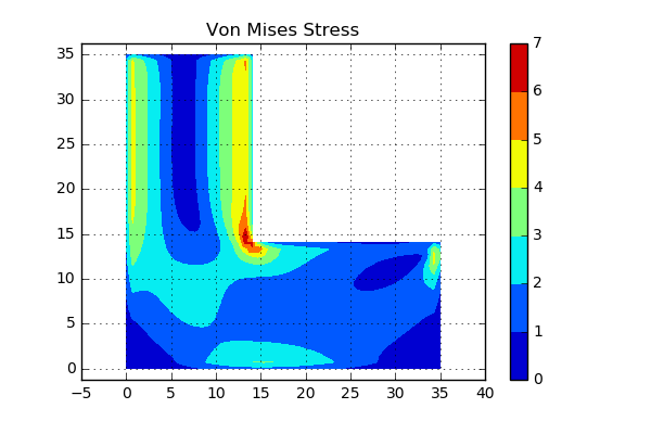
From a pure intuition point of view, the dark blue area (where the stresses are low) would probably be a good place to start to remove material.

Now when we have some expectations on the results after the optimization, why not just run the code almost similar to the ones used in the former blog post and see what comes out? The only thing that has to be updated is the function that creates the dual function and the one computing the final density distribution (which in the former post was the cross section area). Below the code can be seen.

def GetDual(lam,ex,ey,D,rho,q,f,a,nelm,Ed,Vmax):
    
    if lam < 0.0:
        lam = 1e-3
    
    Ck = np.asscalar(f.T*a)
    A1 = []
    A2 = []
    for i in range(nelm):
        ke,ff,area = co.plani4e(ex[i],ey[i],ep,D)
        ci = np.asscalar(np.mat(Ed[i].reshape(1,8)) * ke * np.mat(Ed[i].reshape(8,1)))
        
        xi = np.sqrt(ci*rho[i]**2/(area*lam))
        xi = np.asscalar(xi)
        if xi > 1.0:
            xi = 1.0
        if xi < 1e-6:
            xi = 1e-6
        A1.append( ci*(rho[i]-rho[i]**2/xi) )
        A2.append( area*xi )
        
    # Construct dual function
    psi = np.sum(A2) - Vmax
    
    return psi

With these functions updated, we can now run the main code, as is listed below.

nrIter = 20
rho_mat = np.zeros([nelm,nrIter])
q=3
rho = np.ones(nelm)*0.35
lam=0.1
Ck_vec = []


x0 = 1e-3
for ii in range(nrIter):
    # Set up and solve problem
    K = np.mat(np.zeros((ndof,ndof)))
    for i in range(nelm):
        ke = co.plani4e(ex[i],ey[i],ep,D*rho[i])
        K =  co.assem(Edof[i,1:],K,ke[0])

    (a,r) = co.solveq(K,f,bc[:,0])
    Ed = co.extractEldisp(Edof[:,1:],a)
    
    # Solve duality problem to find new lambda_star
    lam_Star = fsolve(GetDual,x0,(ex,ey,D,rho,q,f,a,nelm,Ed,Vmax))[0]
    AA,Ck,rr = GetRho(lam_Star,ex,ey,D,rho,q,f,a,nelm,Ed,Vmax)
    print('lam_Star: ' + str(lam_Star))
    print('sum(rho): ' +str(np.sum(AA)) )
    print('Ck: ' + str(Ck))
    Ck_vec.append(Ck)
    print('Constraint: ' + str(rr))
    rho = AA
    x0 = lam_Star
    rho_mat[:,ii] = rho
    

One additional thing to notice is that now we are assuming the constraint to be active and thereby solving the dual function. This can be since we now are using the scipy function fsolve instead of the scipy function fmin as we used last time.

Sweet, are you ready to see the results? Below you see a contour plot of the density:

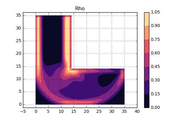
So, what can we say about this? Well, first of all the density is kind of similar to the stress distribution shown earlier. The areas with low stress also show low value of the density. So far so good. However, if we were to use this as a map where to remove material, there are a lot of positions that have a density around 0.5. What to do with those areas, should it be a hole or massive material? What we would like is a more “binary” representation of the density, i.e. keep the material or remove the material. It looks like some conceptual update is needed.

The SIMPsons

How do we “force” the material into this binary kind of behaviour and at the same time do not need to change our code to any great extent? One approach to do this is called SIMP (Solid Isotropic Material with Penalization). The idea is that the effective Young's modulus are related to the density according to:

\[ {\bar E_j} = \rho_j^qE_j\]

where \(q \) is an integer larger than 0. Why does this work? Well, one way to explain is simply to plot the behaviour of the effective Young's modulus. Below a plot can be seen for q=1 and q=3.

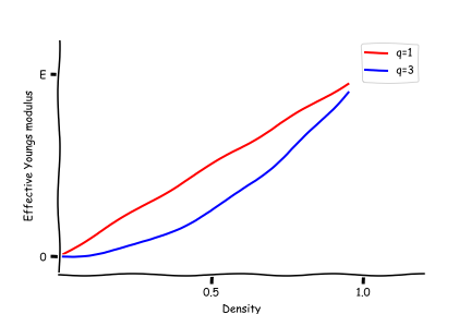
For a density value of 0.5, the obtained stiffness is disproportionately low and therefore such value will be avoided in an optimal solution. It will simply not be an economical use of the material. So, hopefully after adopting the SIMP approach, the structure will have a more binary behaviour.

The next question is: will this SIMP approach result in big changes in the code, since I don't really want that. Well this time we are lucky. The only change that is needed is in the calculation of the effective Young's modulus (but that was kind of obvious), but also in the derivative of the compliance. However, these changes are really small and the code can be seen below.

def GetDual(lam,ex,ey,D,rho,q,f,a,nelm,Ed,Vmax):
    
    if lam < 0.0:
        lam = 1e-3
    
    Ck = np.asscalar(f.T*a)
    A1 = []
    A2 = []
    for i in range(nelm):
        ke,ff,area = co.plani4e(ex[i],ey[i],ep,D)
        ci = np.asscalar(np.mat(Ed[i].reshape(1,8)) * ke * np.mat(Ed[i].reshape(8,1)))*q*rho[i]**(q-1)
        
        xi = np.sqrt(ci*rho[i]**2/(area*lam))
        xi = np.asscalar(xi)
        if xi > 1.0:
            xi = 1.0
        if xi < 1e-6:
            xi = 1e-6
        A1.append( ci*(rho[i]-rho[i]**2/xi) )
        A2.append( area*xi )
        
    # Construct dual function
    psi = np.sum(A2) - Vmax
    
    return psi

OK. lets try to run the updated version of the code as can be seen below and see what turns happens. Here we have not used some fancy criterion to stop the iterations, but rather set a fixed value that will be high enough. An animation of the different iterations can be seen below.

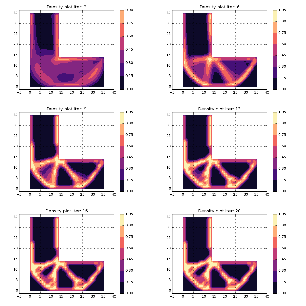
Cool, this looks really nice. Since the shape of the structure is stable during the last iterations, it is assumed that convergens has been reached.

Is finer better?

The above results look really cool, but what if we are not satisfied with the resolution of the results? In general when working with finite element problems, one can always refine the mesh. For most problems (but not all) there exists a point where a finer mesh does not change the results, and here one can refer this to mesh convergence. However, when looking at topology optimization problems, this is in general not the case. If we refine the mesh and perform the optimization again, the numerical result will in general not be a refined improvement of the former results. Rather, the results will differ for every new mesh, i.e. new holes will appear and so forth. This is called mesh dependency. As the mesh gets finer, also the design members get finer.

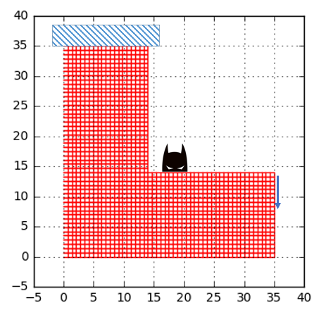
To test this, we simply refine the mesh and run the same code one again. In the picture below, the refined mesh can be seen.

OK, what do the results look like? An animation of the density distribution for the different iterations can be found below.

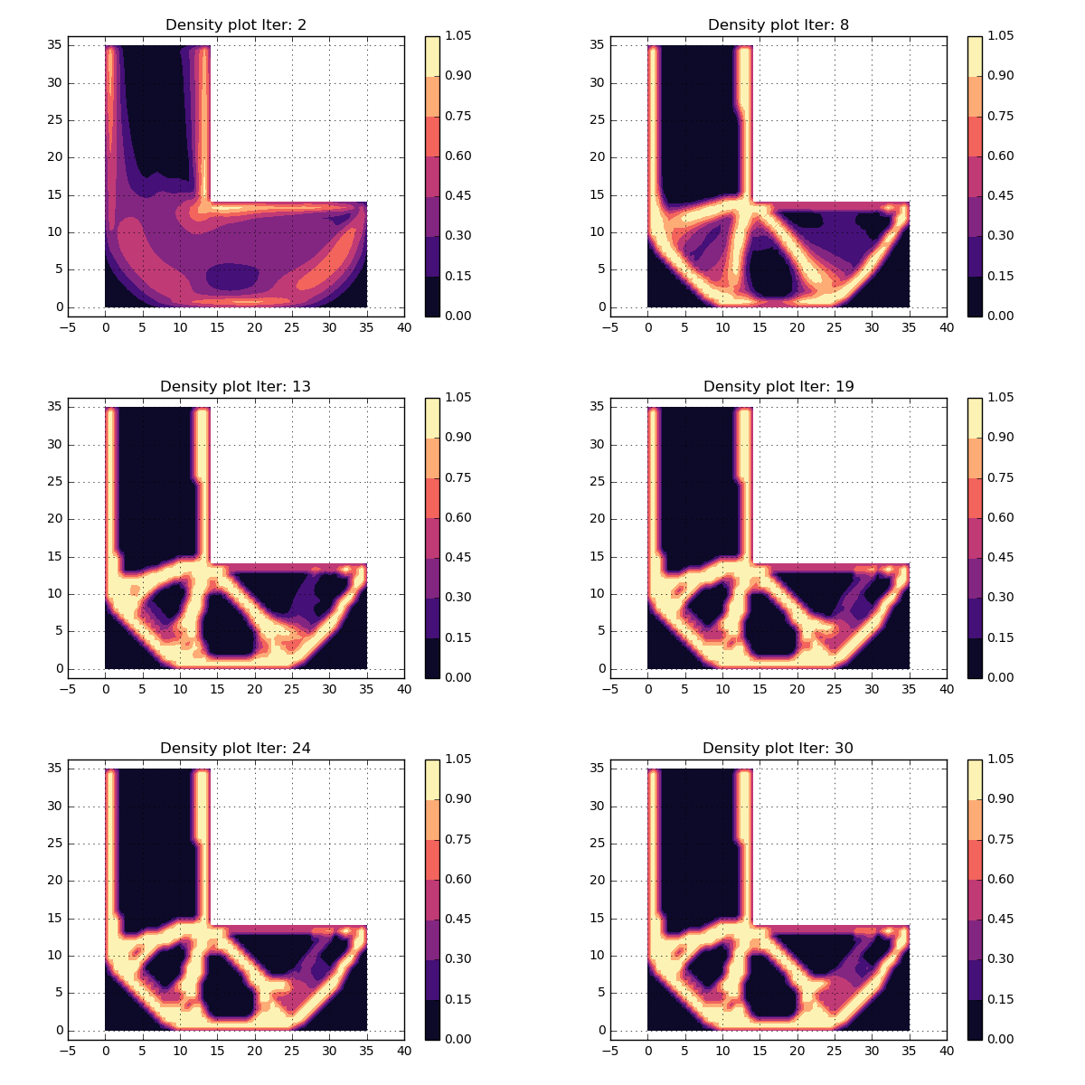
This looks similar but yet different, so some sort of mesh dependency can be seen. We would like to do something about this so let's investigate some ideas.

Filter me this!

As mentioned above, one problem when refining the mesh is that the design members can get really thin. The thickness of these members are more related to the mesh than to physics. In order to reduce this problem, filters can be applied.

A simple by effective approach is to filter the densities. Density filters work by modifying the element density and thereby stiffness to be a function of the densities in a specified neighborhood of an element. The modified element density can be written as:

\[ \rho_{filter} = \rho_{filter}(\rho_i \quad i=1,2,..,nelm) \]

i.e., the modified element density \(\rho_{filter} \) is a function of the neighboring design variables \(\rho_i \).

Some equations may come to mind: Will the total volume of the model change if we apply such a filter? Well, this is in general not a problem since we already have some constraints on the volume. What has to be done is to include the filtered density when checking the volume constraints.

Now, what can this filter function look like? Well one intuitive one could be:

\[ \rho_{filter} = \frac{\sum_{i=1}^{nelm} w_i \rho_i v_i}{\sum_{i=1}^{nelm} w_i v_i } \]

here \(w_i \) is a weighting function, \( v_i \) is the element volume and \(\rho_i \) is as previously discussed the element density. The question is now how to compute the weights? Well, there exists a number of different choices, but here we will go for a Gaussian distribution function defined by:

\[ w_i = e^{-0.5||x_i-x_e ||^2/\sigma_d^2} \]

Note that the weights only have to be computed ones, and this can be done before the optimization starts. The code is not too complicated and can be seen below.

def getWeight(X,ex_mean,ey_mean,sigma_d):
    cc = ((ex_mean-X[0])**2.0 + (ey_mean-X[1])**2.0)/(sigma_d)**2
    return np.exp(-0.5*cc)

Sweet. The last thing that has to be done is to select the value of \( \sigma_d \) wich is realted to the size of the Gaussian bell.

The entire code when adding this filter functionality can be seen below:

nrIter = 30
rho_mat = np.zeros([nelm,nrIter])
q=3
rho = np.ones(nelm)*0.35
lam=0.1
Ck_vec = []
sigma_d = 0.25

rho_filter = np.zeros(nelm)
Weights = np.zeros((nelm,nelm))

ex_mean = np.mean(ex,axis=1)
ey_mean = np.mean(ey,axis=1)


# Create filter weights
for i in range(nelm):
    X = [ex_mean[i],ey_mean[i]]
    wi = getWeight(X,ex_mean,ey_mean,sigma_d)
    Weights[i,:] = wi


x0 = 1e-3
for ii in range(nrIter):
    # Set up and solve problem
    
    # Filter rho before going into FE-solver
    
    K = np.mat(np.zeros((ndof,ndof)))
    for i in range(nelm):
        rho_filter[i] = np.dot(rho,Weights[i,:])/np.sum(Weights[i,:])
        ke = co.plani4e(ex[i],ey[i],ep,D*rho_filter[i]**q)
        K =  co.assem(Edof[i,1:],K,ke[0])

    (a,r) = co.solveq(K,f,bc[:,0])
    Ed = co.extractEldisp(Edof[:,1:],a)
    
    # Solve duality problem to find new lambda_star
    lam_Star = fsolve(GetDual,x0,(ex,ey,D,rho_filter,q,f,a,nelm,Ed,Vmax))[0]
    AA,Ck,rr = GetRho(lam_Star,ex,ey,D,rho_filter,q,f,a,nelm,Ed,Vmax)
    print('==== iter ' + str(ii) + ' ====')
    print('lam_Star: ' + str(lam_Star))
    print('sum(rho): ' +str(np.sum(AA)) )
    print('Ck: ' + str(Ck))
    Ck_vec.append(Ck)
    print('Constraint: ' + str(rr))
    rho = AA
    x0 = lam_Star
    rho_mat[:,ii] = rho
    
rhovalues = np.zeros(edof.max())
elnodes = int(np.size(edof,1))

Now lets try to use three different settings on the \( \sigma_d \) value, i.e. three different radius of Gaussian bell sizes. The result can be seen below:

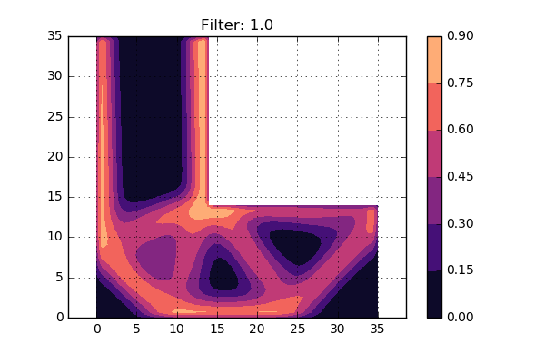
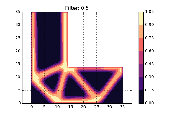
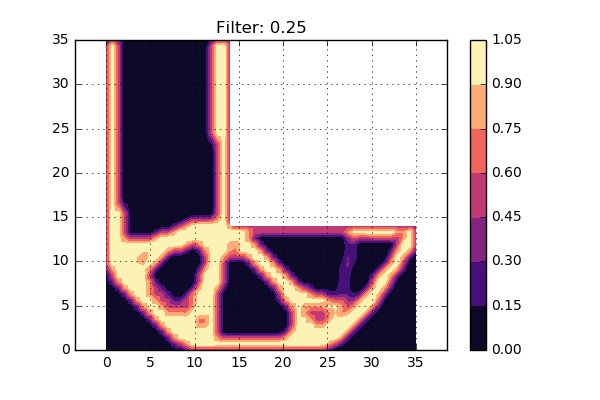
A first conclusion is that the smallest value of \( \sigma_d \) gives a design very similar to the one without a filter. Hmm, perhaps this value is too low then? The largest value of \( \sigma_d \) does not give a very distinct picture, so perhaps this is somewhat too large. The middle value looks to give a crisp and nice density distribution.

Time to conclude

This was the second post on the subject of structural optimization. Here the topology optimization problem was investigated, and it turns out that the code developed for the sizing optimization from the former post only needed some small updates to work for this type of problem. In addition, the mesh dependency was discussed and some strategy (filtering) on how to mitigate this problem.

Hope you enjoyed this post and as usual, if you have questions or comments please contact us.

Reference

P.W Christensen and A Klarbring. An introduction to structural optimization (2009). Springer