Now when the temperature is a positive number (using Celsius), there is only one thing to do: Fire up your grill and do some barbeque! In this post we will have a look at if some finite element modelling using LS-Dyna and python scripting can sharpen your skill at the grill. As mentioned, fire up your grill and fire up some jupyter notebooks.
How to model a chicken...
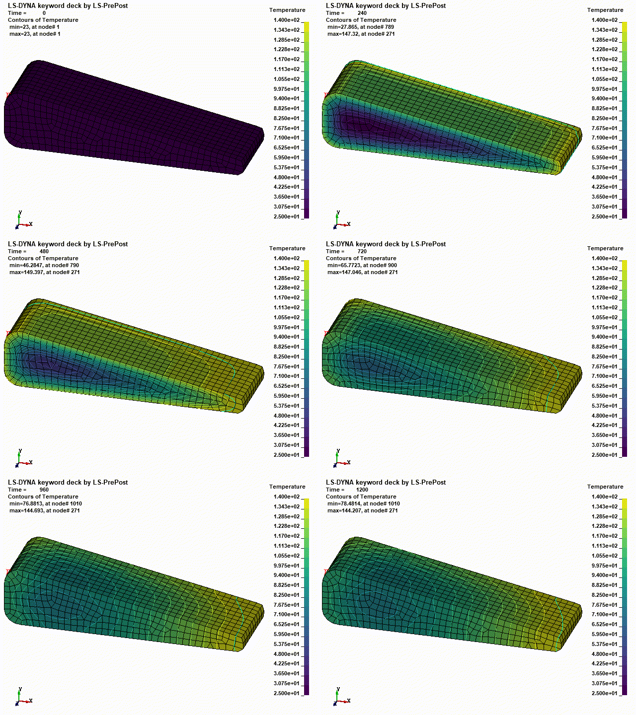
OK, the first thing we will do is to create a model of something that can be put on the grill. I personally really like grilled chicken, so why not try to model that. In the picture below, a finite element mesh of a “chicken breast” can be seen. Here we will be using some symmetry condition (zero flux) and on the remaining boundaries, convection is applied.
The convection condition is simply that the flux is proportional to the difference between the boundary temperature and the ambient temperature:
\[ q = h(T-T_\infty)\]
Here \(q\), \(h\), \(T\) and \(T_\infty\) are the flux, convection coefficient, temperature and ambient temperature respectilvly. We will return to the material parameter \(h\) in a short while.
So far so good! Now let’s have a look at what equations that need to be solved. This in order to figure out what chicken material data is needed. The dynamic temperature problem can be stated below:
\[ \rho C_p \frac{\partial T}{\partial t} = k \nabla^2 T \]
where \(\rho\), \(C_p\) and \(k\) are density, specific heat capacity and thermal conductivity respectively. Next step will be to go hunting for the just mentioned material parameters. I was a bit surprised that there exist quite a lot of academic papers on this subject. From this paper about finite element modelling of cooking a whole chicken, the following material parameters can be found.
| \(k \ W/(m K) \) | \(C_p \ kJ/(kg \ K)\) | \(\rho \ kg/ m^3\) | |
|---|---|---|---|
| Skin | 0.228 | 2.181 | 812 |
| Rib bone | 0.286 | 2.167 | 1040 |
| Round bone | 0.265 | 2.021 | 1040 |
| Breast | 0.549 | 3.667 | 1047 |
| Thigh | 0.534 | 3.645 | 1032 |
Since we are here modelling a chicken breast, we will use that data. In the same paper, also some discussion about the convection parameter \(h\) can be found. This parameter is of course more related to how the chicken will be cooked (boiled, grilled and so on) and also dependent on other parameters. Here we will just use the following value:
\[ h = 166.0 \ W / m^2 \]
So at this point, most of the data for the model has been captured. However, to more in detail capture good grilling practice, the chicken needs to “rest” some time after the grill before going on the plate. At this resting time, the chicken is wrapped in foil (or paper) to let the temperature even out in the meat and also just let it “set”. To model this resting period, the following scaling curve is applied to the parameter \(h\).
Here it is assumed that the time between the grill (\(t_1\)) and wrapping of the chicken (\(t_2\)) takes approximately 100 sec. Let's do the first test run. This time we use a grill temperature of 150 C, chicken that has been prepared at room temperature (initial temperature is 23 C) and a time on the grill before resting for a bit over 8 min (500 sek). A short animation of the temperature distribution over time can be seen below.

Script like a chicken...
Now when we have a working model, it is time to begin leverage using python scripting. As we did in this post, Lasso will be our main path to get access to data produced using LS-Dyna. Let’s start by doing some imports.
import os

from lasso.dyna import D3plot, ArrayType, FilterType, Binout
import numpy as np

import matplotlib.pyplot as plt
import matplotlib as mpl
mpl.style.use('classic')
%matplotlib inline
My biggest concern when serving chicken to my guests is (beside also serving cold beer) that the chicken can not be undercooked. For this reason, it makes sense to track the position with the lowest temperature during the entire grilling process. To get some data to play with, let's run 6 different analysis with some different settings. The different analyses can be seen below. The temperature on the grill is kept constant at 150 C.
| Analysis | Initial temperature (C) | Time on grill (s) |
|---|---|---|
| Run01 | 8 | 200 |
| Run02 | 8 | 400 |
| Run03 | 8 | 600 |
| Run04 | 23 | 200 |
| Run05 | 23 | 400 |
| Run06 | 23 | 600 |
In the first three analyses, the chicken has been taken directly from the fridge and put on the grill, in general not good grilling practice! For the last three, the chicken has reached room temperature before getting on the grill.
Now, let’s write some code that plots the temperature for the coldest position of the chicken during the grilling process. Not that much code is needed for this:
Name = ['Run0'+str(i+1) for i in range(6)]

# Create some plot styles
PlotStyle = {'Run01':'b-','Run02':'b--','Run03':'b-.',
             'Run04':'r-','Run05':'r--','Run06':'r-.'}

# Loop over all analysis
for na in Name:
    # Load d3plot data
    d3plot1 = D3plot(na+"/d3plot",)
    min_temp = []

    # Access the temperature data and find coldest spot for
    # every time step
    for i in range(d3plot1.n_timesteps):
        min_temp.append(np.min(d3plot1.arrays[ArrayType.node_temperature][i]))

    # Plot data
    plt.plot(time,min_temp,PlotStyle[na],lw=2,label=na)

# Put some labels on the axis etc...
plt.legend(loc=2)
plt.xlabel('Time [s]')
plt.ylabel('Temperature [C]')
plt.grid()
and the result can be seen below:
Sweet! The first thing to notice is that the temperature of the coldest position of the chicken will continue to rise after it has been removed from the grill and wrapped. So this is the first lesson to learn: If you are aiming for a particular temperature, you need to get the piece off the grill before it reaches this temperature.
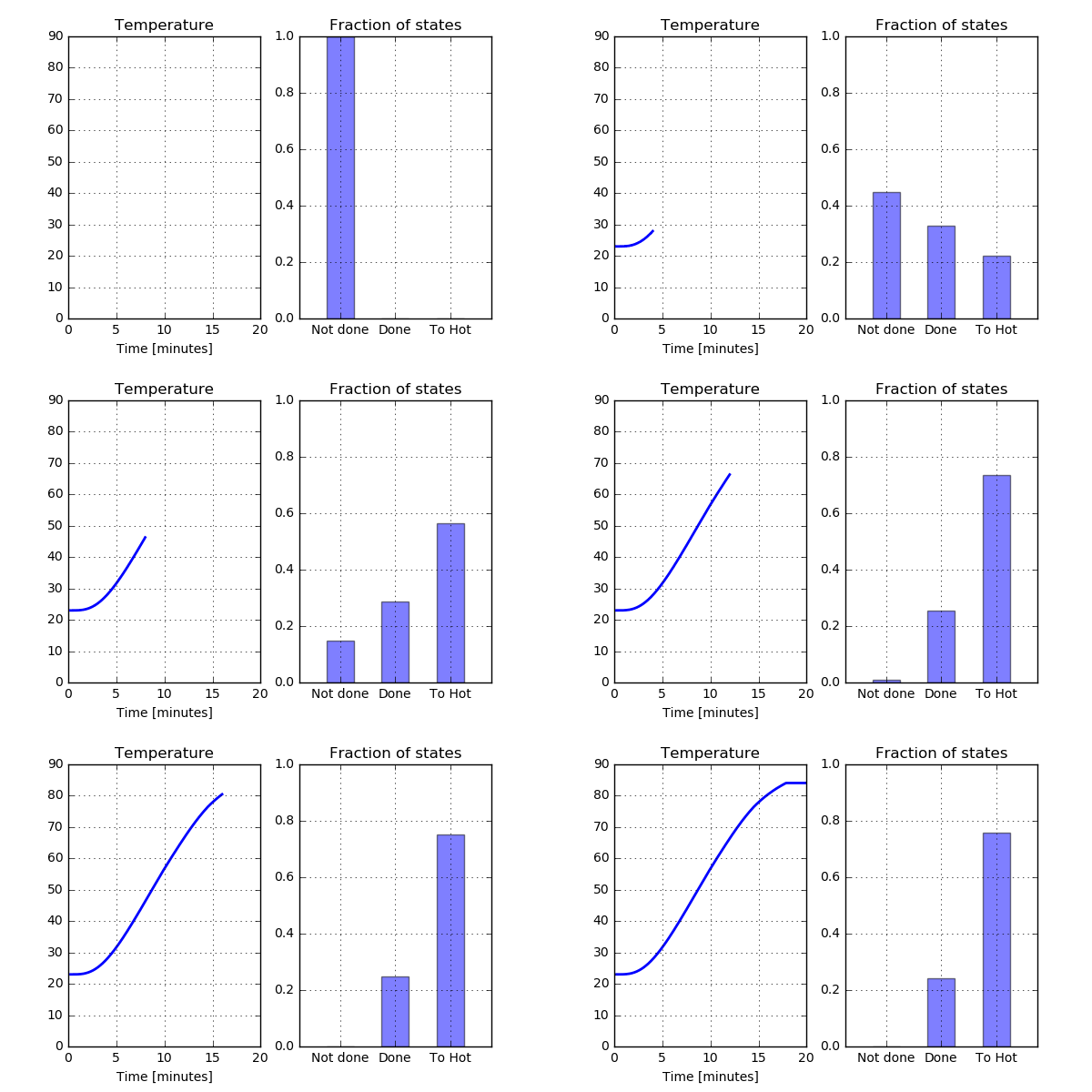
Now let’s investigate the distribution of temperature during the cooking time. To do this let’s investigate the amount of chicken that has reached a certain temperature. Start by defining three categories: Temperature below 70 C would be classified as “Not done”, 70-100 C is classified as “Done” and over 100 C is “Too Hot”. Here the element average will be used. This requires some more coding but still not that bad. Here a number of figures will be saved, and these can later on be used to create a movie (animated gif).
d3plot = D3plot('Run06'+"/d3plot",)
nodeidx = d3plot.arrays[ArrayType.element_solid_node_indexes]
nelm = len(nodeidx)
time = d3plot.arrays[ArrayType.global_timesteps]

min_temp = []

for i in range(d3plot1.n_timesteps):
    Temp = d3plot.arrays[ArrayType.node_temperature][i]

    # Find the min temperature
    min_temp.append(np.min(Temp))

    # Do some plotting
    plt.subplot(1,2,1)
    if i == 0:
        plt.plot(0,min_temp,'b',lw=2)
    else:
        plt.plot(time[:i+1]/60.0,min_temp,'b',lw=2)
    plt.grid()
    plt.xlim(0,20.0)
    plt.ylim(0,90)
    plt.title('Temperature')

    # Compute element average
    ElAvg = []
    for j in range(nelm):
        ElAvg.append( Temp[nodeidx[j]].mean() )
    ElAvg = np.array(ElAvg)

    # Create categories
    NotDone = np.sum(ElAvg < 70)
    OK = np.sum((ElAvg >= 70) & (ElAvg < 100))
    ToHot = np.sum(ElAvg > 100)

    # Do some more plotting
    plt.subplot(1,2,2)
    plt.bar([1,2,3],[NotDone/nelm, OK/nelm, ToHot/nelm],width=0.5,color='b',alpha=0.5)
    plt.xlim(0.5,4)
    plt.xticks([1.25,2.25,3.25],['Not done', 'Done', 'To Hot'])
    plt.ylim(0,1)
    plt.grid()
    plt.title('Fraction of states')
    plt.savefig('Bar_'+str(i))
    plt.clf()
To create an animated gif, the package “imageio” will be utilized. In a few lines of code, the pictures will be turned into an animated gif.
import imageio

filenames = ['Bar_'+str(i)+'.png' for i in range(0,d3plot1.n_timesteps,2)]
images = []
for filename in filenames:
    images.append(imageio.imread(filename))
imageio.mimsave('movie1.gif', images)
Why not take a look at the results for Run06 (initial temperature: 23 C and time on grill: 10 min). Looking at the graph above, this is the analysis with the highest temperature after wrapping. As the lowest temperature at the final state is above 70 C, it is not expected that there will be any part of the chicken that has the status “Not done”. Let’s see what this looks like.

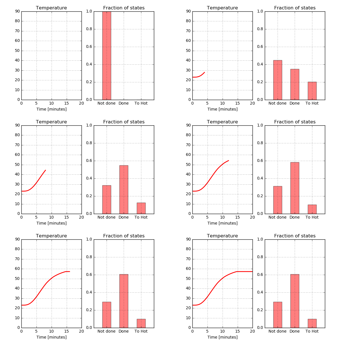
Not too bad. As expected, there is no part of the chicken that has the status “Not done” after approximately 13 minutes. However, a quite large part of the chicken has reached the status “Too hot” indicating that the chicken is a bit overcooked. What does the Run04 look like? Here the temperature is below 70 C for at least some part of the chicken during the entire cooking process, so this is not something I would like to serve to my guests.

This does not look too good. A large part of the chicken has not reached the temperature to be categorized as “Done” so let’s avoid serving this to anyone other than perhaps the cat.
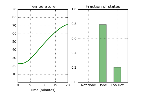
One final exercise before we are done. It happens that I from time to time test to apply the method “Low and Slow” when I am spending time doing BBQ. Why not give that a go? Start by lowering the temperature to 110 C and increase the time on the grill before wrapping to let's say 800 seconds. If this is enough to get the lowest temperature above 70 C, hopefully the part that has reached the “Too hot” category will be smaller. Let’s have a look at the results below:

Must say that this looks really nice. The lowest temperature has reached the 70 C needed to get into the “Done” category and not that large part of the chicken is in the “Too hot” category.
Time to conclude
In this blog post we had a second look at using the Lasso package to access data from a LS-Dyna analysis in python. Here we did some operations on d3plot data in order to show some graphs. For the model of the grilled chicken, I am sure that a lot of improvements can be done. One obvious thing to include is the moisture content. However, to show the use of Lasso, it is my opinion that this model works well.
That is all for this time. As always, please feel free to reach out to us on info@gemello.se.