In this blog post we will revisit a subject I first got in contact with close to 20 years ago. This first contact was kind of bittersweet, since the subject can be really frustrating as well as really satisfying. I am of course talking about the subject of constitutive modelling or the relation between strain and stress. The idea is here to revisit one of the most commonly used models when studying plasticity. If you already find this to be interesting, I can really recommend this book as a starting point.
Life in plastic, it's fantastic
The first model that most of us come in contact with when studying solid mechanics is the linear isotropic one. However, when moving into the field of plastic, some new concepts are needed.
What if the response instead will be nonlinear and plastic? What modifications do we need to do?
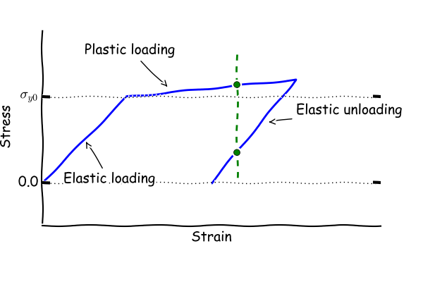
First let's have a look at what caraterice plasticity. One way to do this that's often used is to look at uniaxial tension response where both loading and unloading is displayed. Below one such graph can be seen.

Some fancy things to notice:
- The response is non linear. After loading to \( \sigma_{y0} \) the material characteristics change.
- The total strain does not determine the stress. This is clear when the same level of strain can result in two different levels of stress (green dotted line in graph)
- When unloading, the material do not follow the same path as for loading. In the graph this can be seen since returning to zero stress will result in non zero strain.
To handle these fancy features, some change is needed in the way we formulate the relation between stress and strain. One such approach is to instead formulate how the change in strain relates to the change of stress. Also some additional variables are needed (currently unknown how many) to in some way keep track of the loading history.
\[ \dot{\sigma}_{ij} = \dot{\sigma}_{ij}(\dot{\epsilon}_{ij},\kappa) \]
Given that we now have this view of the constitutive law, let’s have a closer look at one particular model
Who the f..k is von Mises?
From the text above, it looks like a big conceptual change from linear elasticity. This sounds like a difficult task, and yes, it will not be a walk in the park. To somewhat simplify this, we will now get more specific in the choice of constitutive model and why not use the model that you all heard of, the von Mises model. To be a bit more specific, we will look at a special case of the von Mises model: The linear isotropic hardening case.
As some of you might remember, the von Mises model has a “simple” graphical representation where the yield surface can be interpreted as a cylinder with the hydrostatic axis as center point. Below pictures borrowed from Wikipedia can be found.
In the 2D case, this cylinder will turn into an ellipse as shown below:
So what is then the role of this yield surface and how does it fit into the integration of the constitutive equations above? Well, one way to put it is this:
- If the stress state is within the yield surface, then the material behaves elastic.
- If the stress state is on the yield surface (the stress state can not, by definition, be outside the yield surface), the material behaves plastic. This makes our life somewhat more messy…
Now is the time to state a bit more in detail what the model actually looks like and what we need to define to have enough information to create some magic code.
Let’s start by the definition that the total strain can be splitted into one elastic and one plastic part.
\[ \epsilon_{ij} = \epsilon^e_{ij} + \epsilon^p_{ij} \]
As we still assume linear isotropic elasticity, the stress can be written as:
\[ \sigma_{ij} = 2G(\epsilon^e_{ij}+\frac{\nu}{1-2\nu}\epsilon^e_{kk}\delta_{ij}) \]However, at some point further on we will simply state that the stress can be written as:
\[ \sigma_{ij} = D_{ijkl} (\epsilon_{kl} - \epsilon^p_{kl}) \]
Nice! Now for the tricky part. First introduce the yield surface
\[ f = \sqrt{\frac{2}{3} S_{ij} S_{ij}} - \sigma_y \leq 0; \qquad \sigma_y = \sigma_{y0}+H \epsilon^p_{eff} \]
Here \(S_{ij}\) is known as the deviatoric stress, and can be interpreted as the deviation from hydrostatic pressure. The definitions is according to:
\[ S_{ij} = \sigma_{ij} - \frac{1}{3}\sigma_{kk}\delta_{ij} \]
Furthermore, the parameter \(\sigma_{y0}\) is the initial yield stress from unialial tension test and \(H\) is a parameter related to hardeinig. The term \(\epsilon^p_{eff} \) we will return to in just a second or so, but first let’s introduce the evolution of plastic strain. Using what is called associative plasticity, the evolution of plastic strain can be defined as:
\[ \dot{\epsilon}^p_{ij}=\dot{\lambda}\frac{\partial f}{\partial \sigma_{ij}} \]
This looks somewhat confusing. The idea that the evolution of plastic strain would be guided by the gradient of the yield surface is of course not evident. However, experimental data show that this is a good approximation for metals but not so much for soil and rocks. moreover, it the gradient of the yield surface can be seen as the direction of the plastic evolution, the lambda is more related to the magnitude. It is clear that both lambda and the gradint has be to computed in some way to solve this problem.
Now let’s return to the variable \(\epsilon^p_{eff} \). The aim of this parameter is to (in some sense) keep track of the loading history. Looking at the expression for the yield surface, it is clear that the \(\sigma_y\) (which is a linear function of \(\epsilon^p_{eff}\)) represents the radius of the cylinder shown in the figure above. Let’s do the following definition:
\[ \dot{\epsilon}^p_{eff}=\sqrt{\frac{2}{3}\dot{\epsilon}^p_{ij} \dot{\epsilon}^p_{ij}} \]
Sweet! Now we have the model defined and the next step is to take a look at the numeric strategy to do the integration of the constitutive equation.
Let's get phy… no, I mean numerical!
OK, now the fun part begins. So far we have defined the yield function and also the evolution of the plastic strain. Furthermore, an effective quantity containing information of the loading history has been introduced by the effective plastic strain. Now, let's assume that at a certain point in time, we know everything there is to know about a material point under loading. We know the stress and we also know the plastic strain and the effective plastic strain. From this nown state, some additional loading is applied to the material. Our task is now to update all the quantities that were known at the “old” state to this “new” state. We can call this a “stress update”. Not a completely straightforward task, but let’s start by drawing some pictures.
In the above picture you can see the yield surface and also the current stress state, marked by \(\sigma^{(1)}_{ij} \) How do we now handle the change of loading on the material? The stress at the “old” and "new" state can be written as:
\[ \sigma^{(2)}_{ij} = D_{ijkl}(\epsilon^{(2)}_{kl} - \epsilon^{p(2)}_{kl}); \qquad \sigma^{(1)}_{ij} = D_{ijkl}(\epsilon^{(1)}_{kl} - \epsilon^{p(1)}_{kl}) \]
Now simply mash the two equations together gives:
\[ \sigma^{(2)}_{ij} = \sigma^{(1)}_{ij} + D_{ijkl}\Delta\epsilon_{kl} - D_{ijkl}\Delta\epsilon^p_{kl} \]
where:\[ \Delta\epsilon_{kl} = \epsilon^{(2)}_{kl} - \epsilon^{(1)}_{kl} ; \qquad \Delta\epsilon^p_{kl} = \epsilon^{p(2)}_{kl} - \epsilon^{p(1)}_{kl} \]
Not to bad so far! It is clear that the term \( D_{ijkl}\Delta\epsilon_{ij} \) is the stress change that would occur if the step is purely elastic. Moreover, define the “trial” stress as:
\[ \sigma^t_{ij} = \sigma^{(1)}_{ij} + D_{ijkl}\Delta\epsilon_{kl} \]
Using this definition, the stress at the “new” state can be written as:
\[ \sigma^{(2)}_{ij} = \sigma^{t}_{ij} - D_{ijkl}\Delta\epsilon^{p}_{kl} \]
This format gives the opportunity to give a really cool interpretation and computation strategy:
- Compute the trial stress (assuming that the step is purely elastic)
- Compute the value of the yield function at this trial stress, \( f^t \), ones again assuming that the quantities related to plasticity are unchanged during the step.
- If the yield function at the trail stress shows that the response was elastic (\(f^t\lt0\)) then the step was purely elastic and the trail state can be accepted as the “new” state.
- If the yield function at the trail stress shows that the response was plastic (\(f^t \geq 0\)), then the trail stress needs to be corrected by the term \( D_{ijkl}\Delta\epsilon^p_{kl} \).
It looks like we now have a strategy on how to determine if the step is elastic or plastic. The the case of elasticity the task to update the stress and other variables is trivial, but in the case of plasticity, some more work is needed. Let’s start with the term \(\Delta \epsilon^p_{ij} \). Using the evolution of plastic strain it is clear that:
\[ \Delta\epsilon^p_{ij} = \int^2_c\frac{\partial f}{\partial \sigma_{ij}} d\lambda \]
As of definition, up till contact of the yield surface, there will be no evolution of the plastic strain. Hence the lower limit of the integral is the contact point “c”. The upper limit is the “new” state “2”. The problem is that we do only know the term \(\partial f / \partial \sigma_{ij}\) at the contact point, but we can introduce an approxiamtion according to
\[ \Delta\epsilon^p_{ij} = \int^2_c\frac{\partial f}{\partial \sigma_{ij}} d\lambda \approx (\frac{\partial f}{\partial \sigma_{ij}})^* \Delta \lambda \]
where the “*” indicates that the term is evaluated somewhere between the contact point and the “new” stage. So how do we decide this “*”?
Well, one common approach is to use what is called a fully implicit scheme. This is achieved when evaluating the “*” stage at the “new” stage (2). Besides that this choice is numerically stable and accurate, it also has the advantage that we don't need to find the contact state.
OK, but when do we start to write some code??
We have all the parts of the puzzle and “only” need to apply the equations in the last chapter to the von Mises model. The deviatoric stress can be calculated according to:
\[ S_{ij} = 2Ge_{ij}: \qquad e_{ij} = \epsilon^e_{ij} - \frac{1}{3}\epsilon^e_{kk}\delta_{ij} \]
and the evolution of plastic strain can be written as
\[ \dot{\epsilon}^p_{ij}=\dot{\lambda}\frac{\partial f}{\partial \sigma_{ij}} = \dot{\lambda} \frac{3}{2} \frac{S_{ij}}{\sigma_y} \]
The evolution of effective plastic strain can be simplified (after some calculations) to:
\[ \dot{\epsilon}^p_{eff} = \dot{\lambda} \]
Now let's introduce the choice of integration scheme. The stress at stage “2” can then be written as:
\[ \sigma^{(2)}_{ij} = \sigma^t_{ij} - 3G \Delta \lambda \frac{S^{(2)}_{ij}}{\sigma^{(2)}_{eff}} \qquad \sigma^{(2)}_{eff} = \sqrt{\frac{2}{3} S^{(2)}_{ij} S^{(2)}_{ij}} \]
Simply insert this result into the definition of deviatoric stress, the following relations pops up.
\[ S^{(2)}_{ij} = \frac{S^{t}_{ij}}{1+3G\frac{\Delta \lambda}{\sigma^{(2)}_{eff}}} \]
Now I am starting to get a bit tired, but we only have a few more calculations to do before we can fire up python and write some code. The term \( \sigma^{(2)}_{eff} \) needs some more attention. Start by multiplying the right and left side of the equation above with it self, this relation can be found
\[ \sigma^{(2)}_{eff} = \sigma^{t}_{eff} - 3G\Delta \lambda \]
Insert this into the equation above gives:
\[ S^{(2)}_{ij} = S^{t}_{ij}(1-3G \frac{\Delta \lambda}{\sigma^{t}_{eff}}) \]
Allright! The only thing left now is to somehow identify \( \Delta \lambda \) since this is the only unknown left. And you might already have guessed what piece of information we have not utilized yet? Thats right, the yield function. As stated earlier, the yield condition has to be satisfied, i.e.
\[ \sigma^{(2)}_{eff} -(\sigma_{y0} + H\epsilon^{p(1)}_{eff}+H\Delta \lambda) = 0 \]
After a bit more grinding, an (explicit) expression for \( \Delta \lambda\) can be found:
\[ \Delta \lambda = \frac{f^t}{3G +H} \qquad f^t = \sigma^{t}_{eff} - \sigma^{(1)}_y \]
And I think that was it! Now for some coding.
Please, can I start to write some code now??
Now it is finally time to write some code. First out is a sub function that perform the stress update. This sub function takes three input argument, the total strain for the new step, the history variables (in our case the plastic strain and effective plastic strain) and also some material parameters. The outputs from the function are the new stress state, the new history variables and also a variable that indicates if this step was elastic or plastic.
def stress_update_VM(strain,Hist_old,matpar):

    # Material parameters
    E = matpar[0]
    v = matpar[1]
    sy0 = matpar[2]
    H = matpar[3]
    ptype = matpar[4]

    G = E/(2.0*(1.0+v))

    # Initiate old variables
    ep_o = Hist_old[0:4]
    ep_eff_o = Hist_old[4]

    # Define strain vector
    et = np.array([strain[0],strain[1],0.0,strain[2]/2.0])

    # Compute deviatoric part
    tr_et = et[0] + et[1] + et[2]
    eet_dev = et - 1.0/3.0*tr_et*np.array([1.0,1.0,1.0,0.0]) - ep_o

    # Compute trail stress
    St = 2.0*G*eet_dev

    # Compute value of yield function
    SS_t = St[0]**2 + St[1]**2 + St[2]**2 + 2.0*St[3]**2
    sy_t = sy0 + H*ep_eff_o
    sy_eff_t = np.sqrt(3.0/2.0*SS_t)
    f_t=sy_eff_t-sy_t


    # Elasticity
    if (f_t < 0):
        Hist_new = Hist_old
        D_ats = co.hooke(3,E,v)
        tr_es=2.0*G*(1.0+3.0*v/(1.0-2.0*v))*tr_et
        es = St + 1.0/3.0*tr_es*np.array([1.0,1.0,1.0,0.0])
        es_mat = D_ats * np.matrix(et).T
        sy = sy_t
        State = 'Elastic'

    # Plasticity
    else:
        # Compute delta lambda
        dl = f_t/(3.0*G + H)

        # Update variables
        ep_n = ep_o + dl*St/sy_eff_t*3.0/2.0
        ep_eff_n = ep_eff_o + dl
        sy = sy0 + H*ep_eff_n

        # Compute new elastic strain
        ee_n=et-ep_n
        tr_een = ee_n[0]+ee_n[1]+ee_n[2]

        S = St*(1.0-3*G*dl/sy_eff_t)
        tr_es=2.0*G*(1.0+3.0*v/(1.0-2.0*v))*tr_een
        es = S + 1.0/3.0*tr_es*np.array([1.0,1.0,1.0,0.0])

        State = 'Plastic'

        # Update history variabels
        Hist_new = np.array([ep_n[0],ep_n[1],ep_n[2],ep_n[3],ep_eff_n])


    # Return stuff
    return es, Hist_new , State
OK, a bit of code but the equations follow the calculations that were done above. In this blog post we will simply provide a new strain state to the sub function and let it do some magic. We will not connect this to any finite element code at this moment, however this will be done in later posts. For this reason, the loading condition will be rather simple and can be seen in the picture below. Strain is applied in one direction when all the other strain components remain zeros.
Some material parameters are also needed. Below you find a table where this can be found. The hardening parameter \( H \) will initially be set to zeros in order to simulate ideal plasticity.
| Material properie | Value |
|---|---|
| \( E \) | 210e3 |
| \( \nu \) | 0.3 |
| \( \sigma_{y0} \) | 250 |
| \( H \) | 0 |
The loading will be an increase of strain until we are well within the plastic area, followed by some unloading.
Hist_old = np.array([0.0,0.0,0.0,0.0,0.0])
sy0 = 250.0
H = 0.0
E,v = 210e3, 0.3
ptype = 3
matpar = [E,v,sy0,H,ptype]

#strain_xx = np.arange(0,0.004,1e-4)
strain_xx1 = np.linspace(0,0.004,180)
strain_xx_2 = np.zeros(180)
strain_xx_2[120:] = np.linspace(0,0.002,60)
strain_xx = strain_xx1 - strain_xx_2

ep_eff_v = []
es_v = []
State_v = []

es1 = []
es2 = []
es3 = []
sy_v = []
for i in range(len(strain_xx)):

    strain_test = np.array([strain_xx[i],0.0,0.0])


    es,Hist_new,sy,State = stress_update_VM(strain_test,Hist_old,matpar)
    es1.append(es[0])
    es2.append(es[1])
    es3.append(es[2])
    sy_v.append(sy)
    es_v.append(es[0])
    State_v.append(State)
    ep_eff_v.append(Hist_new[-1])
    Hist_old = Hist_new
Let's run the code and then have a look at the results...
Show me some results
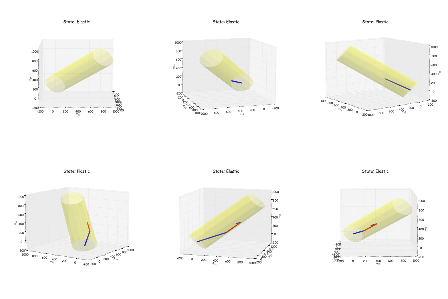
Even though the loading condition is simple, some cool results can be obtained. Here we will have a look in stress space and see how the stress state reacts when it hits the plastic area. Since the material parameters are set so as to simulate ideal plasticity, it is expected for the yield surface not to grow as we enter into the plastic area. It is also expected that the stress state will stay on the yield surface when the loading is increased, and then move back into the elastic area when unloading is performed. Below an animation of the stress state can be seen. Note that blue dots indicate elastic loading and red dots indicate plastic loading.

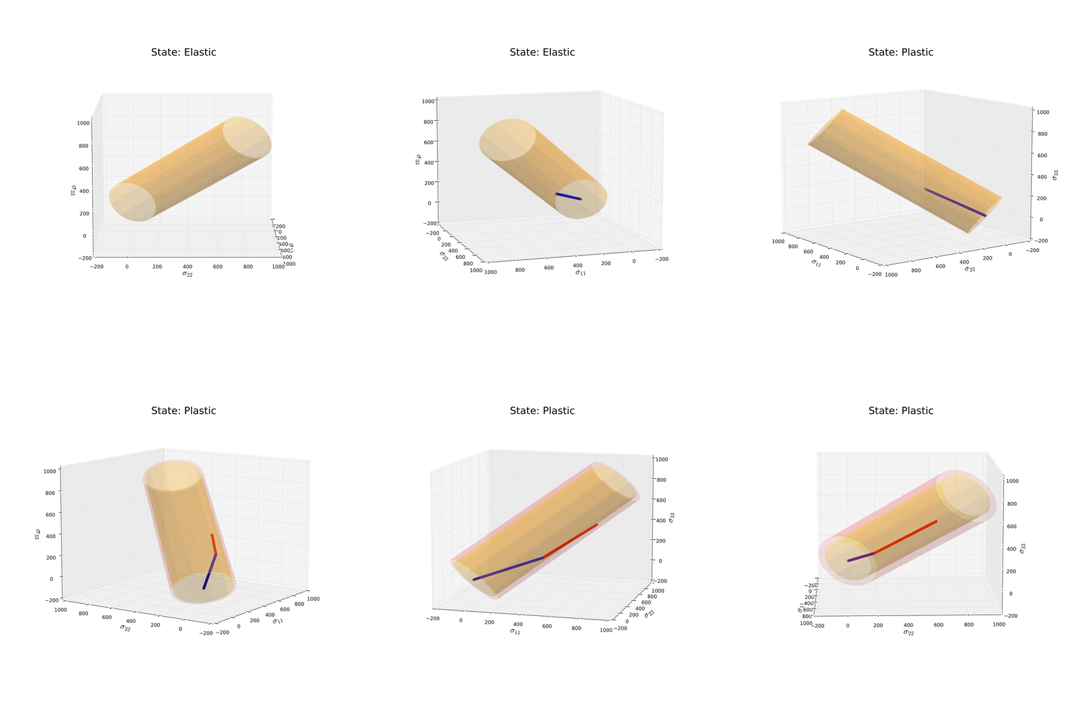
Not too bad! The animation shows what was expected for this loading condition and material parameters. Now let’s change some things and run one more simulation. Start by including some harding. By doing so, it is expected that the radius of the yield surface will grow as plastic deformation occurs. The unloading is for this example not included. The original shape of the yield surface will be yellow and the “new” shape of the yield surface will be red.

Time to conclude
In this blog post we have looked into one of the most commonly used material models for metals. Even though this is considered as a simple one, the implementation is far from trivial. We will return to this model in the not too far future, where we will implement this code into a finite element framework.
That is all for this time. And as always, please feel free to reach out to us on info@gemello.se.