This is the first blog post on the subject “material calibration”. As the name suggests, this subject deals with the problems of extracting material parameters from a constitutive model to fit some intended behaviour (from experimental data or other). In this first blog post, we will actually not perform any material calibration but we will investigate some activities that can be performed even before experimental tests are collected.
Making it fit?
The concept for material calibration (or parameter identification) can be grasped by a pretty simple example. Below a figure can be seen where the data is from a uniaxial tension test.
The recorded output from the test was here the force and displacement. The task for the material calibration activity is now to find the best model and best set of parameters that can recreate these experimental results.
This does perhaps not appear to be that complicated, but some questions come to my mind:
- What does “best” mean in terms of fit?
- Is it even possible to determine all material parameters from the given test data?
Sensitivity
So even before collecting material test data, are there some activities that can be done in order to have a higher chance of succeeding with the material parameter identification? Well, if we know nothing about the material, then this is perhaps not so easy. However, if we know that we are starting out with some pre-defined material model to fit the data to, some activities can be done.
Starting by just investigating what data is needed to perform a finite element analysis, most of the time the following data is needed:
- Geometry
- External loading
- Boundary conditions
- Choice of constitutive law and suitable material parameters
In addition, some observed responses are also recorded as output from that model. In this case, the output is only useful if the same type of output can be collected from a later experimental setup. One such output can be deformation of a certain point of the geometry, but also magnitude of external loading can be recorded.
So, let’s start by simply setting up a simulation of a uniaxial tension test. The recorded output will be the external loading and also the displacement of the loaded part of the body. Due to symmetry only a quarter of the geometry is modelled. In the figure below, the geometry can be seen as well as an example of output.
The used material model here will be a von Mises model with mixed hardening, a model that requires five material parameters (material *MAT_PLASTIC_KINEMATIC in LS-Dyna).The material parameters as well as the initial values can be seen in the table below.
| Material properie | Value |
|---|---|
| E (Young's modulus) | 207000.0 |
| pr (Poisson's ratio) | 0.3 |
| sigy (Yield stress) | 350 |
| etan (Hardening parameter) | 2000 |
| beta (Ratio isotropic/kinematic hardening) | 0.5 |
Now for the fun part. A reasonable question to ask would be: How will the output response change if the material parameters are changed? This can be found by calculating the relative response sensitivity. This is defined by:
\[ l_i = \frac{\partial r}{\partial \kappa_i} \kappa_i \qquad i=1,2,3... \]
where \(r\) is the response from the simulation and \(\kappa_i \) is the material parameter with number \(i\). The differentiation with respect to the material parameter can be done in a numerical fashion according to:
\[ \frac{\partial r}{\partial \kappa_i} \approx \frac{r(\kappa + \Delta \kappa) - r(\kappa)}{\Delta \kappa} \]
Nice! Now let’s start to write some code.
It's coding time!
It's time to start up a Jupyter notebook and write some code. Let’s start by creating some folders where the simulation data can be stored.
# Create some folders
wai = os.getcwd()
Name = ['Run0'+str(i+1) for i in range(6)]
for na in Name:
    os.mkdir(wai+os.sep+na)
Sweet! Now we have six folders to store some data in. Why we created six folders and not any other number is because we will need one “reference” simulation as well as five additional simulations where the material parameters are perturbed in order to calculate the sensitivities. In order to run the simulations, a parameter file needs to be created. This is done using the function below
def printPar(Par,Name):

    f = open(wai+os.sep+Name+os.sep+'Parameter.key','w')
    f.write('*KEYWORD\n')
    f.write('*parameter\n')
    f.write('RE, %5.1f, Rpr, %5.2f, Rsigy, %5.1f, Retan, %5.1f\n' % (Par[0],Par[1],Par[2],Par[3]))
    f.write('RBeta, %5.1f\n' % (Par[4]))
    f.write('*INCLUDE\n')
    f.write('..'+os.sep+'01-Main.key\n')
    f.write('*END')
    f.close()
With this function in place, we can now create all the needed parameter files. As can be seen below, the perturbation is here set to 5% of the material parameter value.
# Create some files
Par1 = np.array([207000.0, 0.3, 350.0, 2000.0, 0.5])

# Print Original Parameter file
printPar(Par1,Name[0])

for i in range(5):
    pert = np.zeros(5)
    pert[i] = 0.05
    Par = Par1 + pert*Par1[i]

    # Print Parameter file
    printPar(Par,Name[i+1])
All the parameter files are now created, and the next thing is to run all the six simulations. After this is done, the next step will be to extract some data from the simulation results. For this purpose, lasso.dyna will be used. Ones this package is imported, a small function can be created to read the reaction forces.
from lasso.dyna import D3plot, ArrayType, FilterType, Binout

def GetResponce(Foldername):
    binout = Binout(wai+os.sep+Foldername+os.sep+"binout")
    x_force_0 = -np.sum(binout.read('spcforc','x_force')[:,:5],axis=1)
    return x_force_0
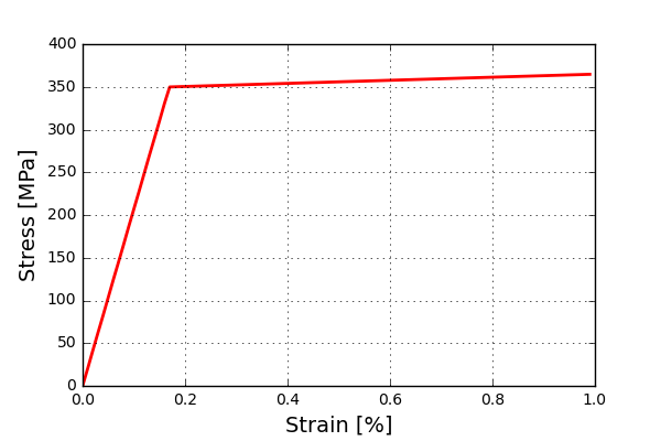
First, let’s have a look at the response from the reference settings. Below the stress vs strain relation can be seen. As expected, the model shows linear hardening after the initial yielding.
From here, let’s read the results from all simulations and construct the sensitivities.
r0 = GetResponce('Run01_Exp')
r1 = GetResponce('Run02_Exp')
r2 = GetResponce('Run03_Exp')
r3 = GetResponce('Run04_Exp')
r4 = GetResponce('Run05_Exp')
r5 = GetResponce('Run06_Exp')

l1 = (r1 - r0)/0.05
l2 = (r2 - r0)/0.05
l3 = (r3 - r0)/0.05
l4 = (r4 - r0)/0.05
l5 = (r5 - r0)/0.05
Not too bad. Let’s have a look at what the difference sensitivities looks like when plotted.
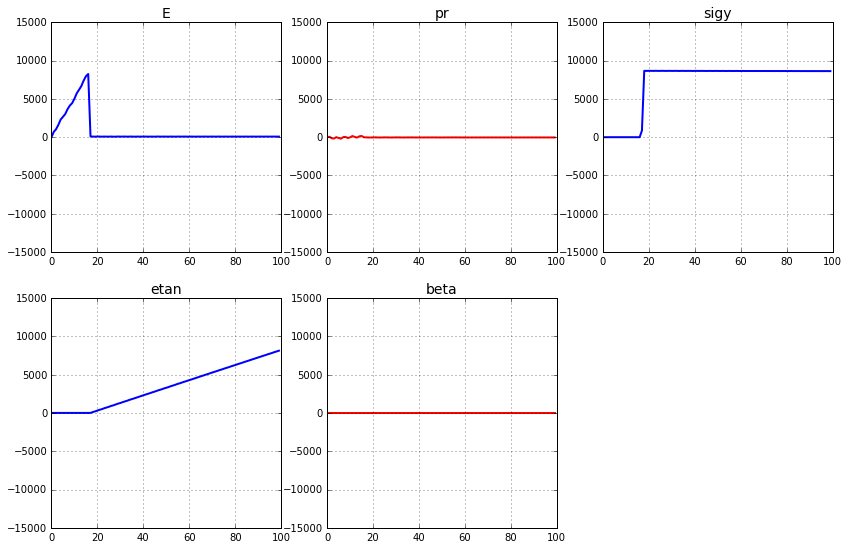
Wow, these results are really interesting! The first thing I noticed was that for two of the parameters, “pr” and “beta”, it looks like a change in this parameter does not affect the response at all, since the results are just flat lines at a value of zero. OK, so that does this mean? Well, it means that it would not be possible to determine the values of these parameters, since no matter what value the parameters will take, it will not affect the response.
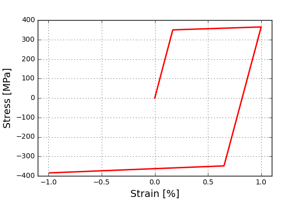
So, what can we do to improve this? Well one thing that we can do is to include more data in the response. One idea could be to change the loading history to also include deloading and compression loading. The response can look like this:
What would then the sensitivities look like? Well an updated graph can be seen below.
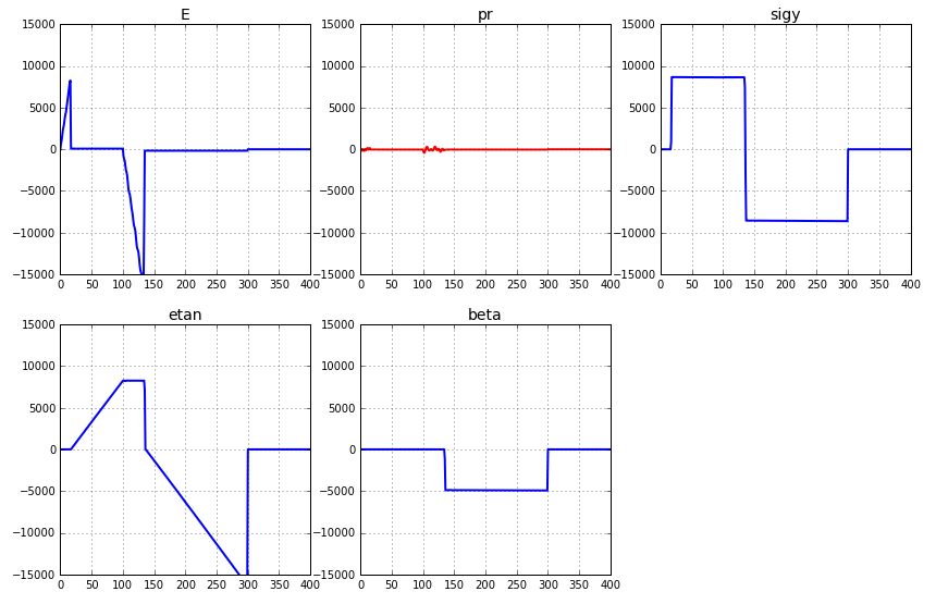
Nice! It appears that the investment in collecting more data for the response has paid off. The “beta” parameter does now contribute to changes in the response. Are we surprised? Well, not really. The “beta” parameter is related to isotropic/kinematic hardening of the material model, and this will only be visible when reversed yielding occurs.
But what about the last parameter “pr”? What can we do to get hold of this parameter? Well, I think you all have guessed what we can do. Why not also include the deformation perpendicular to the loading direction? Some smaller changes to the function returning the response has to be made, see below.
def GetResponce(Foldername):
    binout = Binout(wai+os.sep+Foldername+os.sep+"binout")
    x_force_0 = -np.sum(binout.read('spcforc','x_force')[:,:5],axis=1)
    y_disp_0 = binout.read('nodout','y_displacement')[:,4]
    return x_force_0,y_disp_0
And this is what the sensitivity looks like for this response. Here only the loading up to initial yielding is investigated.
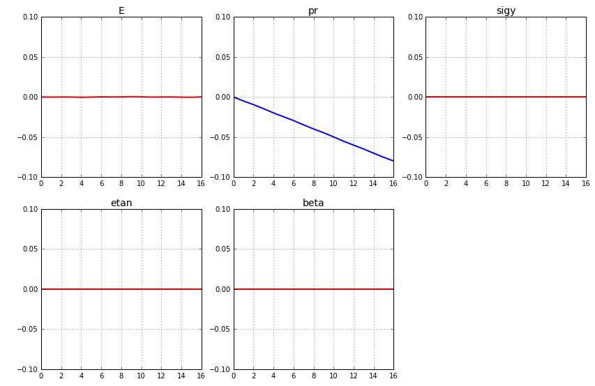
Allright! Now we have come to the conclusion that by combining the responses discussed above, it would be possible to actually calibrate all the five material parameters. For all of you that have a clear interpretation of the different material parameters included in this model, the result should come as no surprise at all.
Time to conclude
This was the first post on the subject of material calibration. Here we did not actually perform any material calibration but we did something that also is of great importance: to investigate what experimental data is needed to calibrate the used model. We will come back to the subject of material calibration at least a few more times in the near future.
Well, that's all for this time. And as always, please feel free to reach out to us on info@gemello.se.