In this post we are once again back at the golf course. In two previous blog posts we have investigated the physics of putting and also done some fun investigations when it comes to robustness. This time we will have a look at the more impressive (if done correctly) part of the golf game, namely the tee shot.
A drive for show, a putt for dough
If you ever have played the game of golf, you may have heard the expression “A drive for show, a putt for dough”. The meaning is that even though an impressive drive will give you lots of credit, to be a good putter will give you a lower score. Today we will just ignore this statement (which by the way may actually not be true) and focus on the fun parts, to hit BOMBS. So let’s watch the man who hits a lot of bombs and then get into the physics.
Let's get airborne
In contrast to what some presidents may think, it is actually partial differential equations that rules the world. This example of “projectile motion” is no exception, and to show that let’s start to look into the most simple example: The classic parabolic motion.
This is an example that I am pretty shue a lot of you have solved using a pen and paper. The starting point of the example is a golf ball that has an initial velocity and a direction. In this case, we simply ignore all acting forces, except gravity, on the ball during the time it spends in the air. Let’s utilize a coordinate system where the x-axis is parallel to the ground in the direction of the drive, y-axis is in the opposite direction as gravity and z-axis is orthogonal to the x- and y-axis. In this case, only forces in the y-direction are active i.e.
\[ \sum F_y = m\ddot{y} \]
or more explicit:
\[ m\ddot{y} = -mg \]
Of course, this would be easy to solve using pen and paper, but here we will use a numerical strategy to solve this problem. This to make our life somewhat simpler as we will move towards more advanced examples.
Start by doing the “regular” imports.
import numpy as np
from scipy.integrate import odeint

import matplotlib.pyplot as plt
import matplotlib as mpl
mpl.style.use('classic')
%matplotlib inline
To solve this differential equation, we will utilize the scipy function “odeint” that can be found in the scipy.integrate module. This function solves a system of ordinary differential equations using lsoda from the FORTRAN library odepack. More specific, the initial value problem for stiff or non-stiff systems of first order ode-s are solved on the format
\[ \dot{\boldsymbol x} = f(\boldsymbol x,t,...) \qquad \boldsymbol{x}(t=0) = \boldsymbol{x}_0 \]
So our task is simply to provide the first time differentiation for this function. Since we also have second differentiations we are required to do a “trick” by introducing the following variables.
\[ \boldsymbol{x} = [x,\dot{x},y,\dot{y},z,\dot{z}] \]
And by this if directly follows that:
\[ \dot{\boldsymbol{x}} = [\dot{x},\ddot{x},\dot{y},\ddot{y},\dot{z},\ddot{z}] \]
Now it is time to write some code for this first simple example. Start to define the time differentiation
def flights(x,t):
    xprime = np.zeros(6)

    # X-direction
    xprime[0] = x[1]
    xprime[1] = 0.0

    # Y-direction
    xprime[2] = x[3]
    xprime[3] = -9.81

    # Z-direction
    xprime[4] = x[5]
    xprime[5] = 0.0

    return xprime
That was simple enough. Let’s have a look at the code that solves this problem. Here we use an initial ball velocity of 160 mph (representative number for a good golfer) and a launch angle of 45 deg. We also assume no velocity component in the z-direction.
v0 = 72.0 # 160 mph ball speed
alpha = 45.0
v0x = v0*np.cos(np.radians(alpha))
v0y = v0*np.sin(np.radians(alpha))

x0 = [0,v0x,0,v0y ,0,0]
t = np.arange(0,12.0,0.01)
wsolv = odeint(flights,x0,t)


ind = np.min(np.where(wsolv[:,2] < 0.0)[0])

plt.plot(wsolv[:ind,0],wsolv[:ind,2])
plt.axis('equal')
plt.xlabel('x [m]')
plt.ylabel('y [m]')
plt.grid()
And the resulting graph can be seen below.
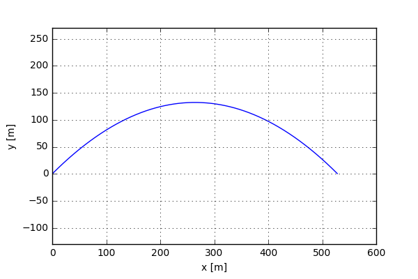
This looks a lot like the classic parabolic motion that I solved back in school. Now Now, let’s increase the complexity a bit. To do this we can introduce the forces coming from aerodynamic drag also known as air resistance. On a general level the equation of motion can be written as:
\[ m \ddot{\boldsymbol{x}} = \boldsymbol{F}_{gravity} + \boldsymbol{F}_{drag} + \boldsymbol{F}_{Magnus} \]
The \( \boldsymbol{F}_{Magnus} \) we will come back to later and is for now assumed to be zero. The air resistance can be calculated using the equation shown below
\[ \boldsymbol{F}_{drag}=\frac{1}{2}C_D\rho A \boldsymbol{v}^2 \]
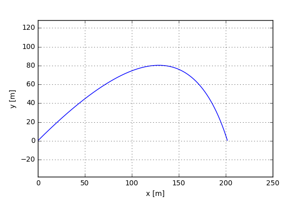
where \( C_D\), \( \rho \), \(A\) and \(\boldsymbol{v}\) are drag coefficient, air density, surface area and velocity, respectively. Some code related to this problem can be seen here.
def flights_SB(x,t):
    # Parameters
    C_d = 0.3
    rho = 1.225 # kg/m3
    D = 42.67e-3 # m
    m = 0.04569 # kg
    A = np.pi*D**2/4

    R = 0.5*C_d*rho*A

    xprime = np.zeros(6)

    # X-direction
    xprime[0] = x[1]
    xprime[1] = -R/m*x[1]**2

    # Y-direction
    xprime[2] = x[3]
    xprime[3] = -9.81-R/m*x[3]**2

    # Z-direction
    xprime[4] = x[5]
    xprime[5] = -R/m*x[5]**2

    return xprime
Once again we use an initial velocity of 160 mph and a launch angle of 45 deg.
v0 = 72.0 # 160 mph ball speed
alpha = 45
v0x = v0*np.cos(np.radians(alpha))
v0y = v0*np.sin(np.radians(alpha))

x0 = [0,v0x,0,v0y ,0,0]
t = np.arange(0,12.0,0.01)
wsolv_SB = odeint(flights_SB,x0,t)


ind = np.min(np.where(wsolv_SB[:,2] < 0.0)[0])

plt.plot(wsolv_SB[:ind,0],wsolv_SB[:ind,2])
plt.xlabel('x [m]')
plt.ylabel('y [m]')
plt.axis('equal')
plt.grid(
And as can be seen in the graph below, the impact of the air resistance is quite big. The path of the ball looks different as well as the total distance.
Now let’s add some additional complexity. This can be done by introducing Magnus forces to acting on the ball. Let's look at a backspin and how it affects the flight of a golf ball. When backspin is placed on a golf ball it will allow the ball to gain loft and have a longer fight. When the ball spins it directs air upwards in front and downward behind it, creating a pressure difference. The pressure difference pushes the ball upward allowing the ball to stay in fight for greater time, this is called the Magnus Force.
The Magnus force lifting the ball is caused by the rotation and the velocity of the ball. The rotation causes air disturbances perpendicular to the direction of the angular velocity causing the direction of flight is altered perpendicular to the linear velocity. This relationship shows that the Magnus force is calculated using a cross product.
\[ \boldsymbol{F}_M = S(\boldsymbol{\omega} \times \boldsymbol{v}) \]
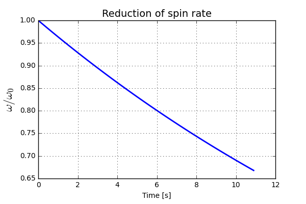
Here \(S\), \(\boldsymbol{\omega}\) and \( \boldsymbol{v} \) are Magnus coefficient, angular velocity and velocity, respectively. Moreover, it is here assumed that the spin rate will slightly decrease during the time the golf ball is in the air. This is done using the following equation
\[ \omega = \omega_0 e^{-t/t_0} \]
Here the constant \(t_0\) is set to get an approximate reduction of 20% after 6 seconds of air time. The reduction of spin rate can be seen in the plot below.
OK, nice! Let’s put this together where we include “all” forces acting on the golf ball. The code looks like this.
def flights_3DPar(x,t,w0i,w0j,w0k,C_d,s):
    # Parameters
    rho = 1.225 # kg/m3
    r = 0.0213 # m
    m = 0.04569 # kg
    A = np.pi*r**2

    R = 0.5*C_d*rho*A

    # Magnus
    M = s/m

    wi = w0i*np.exp(-t/27.0)
    wj = w0j*np.exp(-t/27.0)
    wk = w0k*np.exp(-t/27.0)

    xprime = np.zeros(6)

    # X-direction
    xprime[0] = x[1]
    xprime[1] = -R/m*x[1]**2 + M*(wj*x[5]-wk*x[3])

    # Y-direction
    xprime[2] = x[3]
    xprime[3] = -9.81-R/m*x[3]**2 + M*(wk*x[1]-wi*x[5])

    # Z-direction
    xprime[4] = x[5]
    xprime[5] = -R/m*x[5]**2 + M*(wi*x[3]-wj*x[1])

    return xprime
Now it is time to put his code to the test. Let’s start by investigating how the spin rate affects the ball flight. Our intuition would be that as the spin rate increases, so will the “lift” force of the ball. As the lift increases, so will the carry distance. However, at some point the spin rate will be too high resulting in a shorter carry distance. So, keeping the initial velocity and launch angle constant, try out some different spin rates and see how this affects the ball flight. The code looks like this
v0 = 82.0 # 160 mph ball speed
alpha = 12.

ang = [150,260,340]
dist = []


for a in ang:

    wi = 0
    wj = 0
    wk = a

    v0x = v0*np.cos(np.radians(alpha))
    v0y = v0*np.sin(np.radians(alpha))

    x0 = [0,v0x,0,v0y ,0,0]
    t = np.arange(0,14,0.01)
    wsolv_3D = odeint(flights_3Dspin,x0,t,args=(wi,wj,wk,))


    ind = np.min(np.where(wsolv_3D[:,2] < 0.0)[0])

    print(wsolv_3D[ind,0]/0.9)
    dist.append(wsolv_3D[ind,0])
    plt.plot(wsolv_3D[:ind,0],wsolv_3D[:ind,2])
    plt.axis('equal')
    plt.xlim(0,330)
    plt.grid()

plt.xlabel('x [m]')
plt.ylabel('y [m]')
The resulting ball flight can be seen here
Not too bad. It looks like our intuition was right. However, the drag coefficient and Magnus coefficient can most likely be investigated in a bit more detail. This since the height of the ball is a bit too high to be fully realistic.
Time to conclude
In this blog post we have had a look at what forces are acting on a golf ball when flying airborne. The different categories of forces are all modeled using the simplest possible approach. The result looks to be in line with our intuition. However, some coefficient values probably need to be more closely investigated to generate a bit more realistic results. This will be the scope of the next blog post on the same subject.
As always please feel free to contact us at info@gemello.se.
So, until the next time, Fore!