Gemello Engineering AB - Compute This!

So, time for a new blog post. In this blog post we are going to have a look at a classic problem in optimization called the traveling salesman problem

The traveling salesman problem

The traveling salesman problem is formulated something like this:

Given a list of cities and the distances between each pair of cities, what is the shortest possible route that visits each city exactly once.

(Sometimes it is also needed to return to the city you started in but we are going to ignore this part here). So there might be several reasons for doing so:

To be environmental friendly since you reduce the amount of fuel needed.
More efficient so in the long run you can visit more cities and do more salesman stuff
Or maybe, you just have a really annoying college so you would like to minimize the time spent together in the car.

Now when the problem at hand is formulated it sounds like the first thing we need to do is to generate some map with cities so let’s fire up a jupyter notebook and start some coding!

As usual we start with the “standard” imports

import numpy as np
import matplotlib.pyplot as plt

import seaborn as sns
sns.set(context='talk')

Now, let’s generate coordinates for 10 different cities using the numpy.random.uniform function.

nr_cities = 10
city_coords = np.random.uniform(low=0,high=100,size = (nr_cities,2))

Let's plot the coordinates for these 10 cities

plt.figure(figsize=(10,10))
plt.scatter(city_coords[:,0],city_coords[:,1],s=500,c=np.arange(0,nr_cities),edgecolor='k',cmap='tab10')

plt.axis('equal')
plt.xlabel('X-Coordinates')
plt.ylabel('Y-Coordinates')
plt.title(str(nr_cities) + ' Cities')
plt.show()

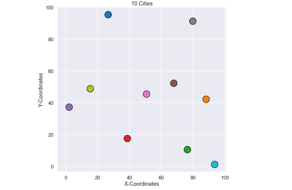
OK, now we have something to work with. Let’s start by solving the traveling salesman problem for these 10 cities using a brute force approach.

Use the (brute) force

A brute force solution is often a quite simple solution method since it. but before we try to find the actual solution to the problem it is obvious that we need a helper function that calculates the total distance we will travel when visiting the cities in a specific order.

def total_distance(city_coords,path):
    dist = 0
    for i in range(0,len(city_coords)-1):
        
        idx_1 = path[i]
        idx_2 = path[i+1]
        dist = dist + np.sqrt((city_coords[idx_1,0]-city_coords[idx_2,0])**2 + 
                              (city_coords[idx_1,1]-city_coords[idx_2,1])**2)
        
    return dist

Here the path contains every number between 0 and 9 and represents the order we visit the different cities. OK, so far so good. Now it is time to use the brute force to find the shortest path and to do so we “just” loop over all possible permutations of a vector that contains the numbers from 0 to 9. For this we use the intertools package and it looks something like this

import itertools
permut_array = np.array(list(itertools.permutations([0,1,2,3,4,5,6,7,8,9])))

dist_vector = []

genome = np.arange(0,nr_cities)
for i in range(0,len(permut_array)):
    path = permut_array[i]
    dist_vector.append(total_distance(city_coords,path))

best_path = permut_array[np.where(dist_vector==np.min(dist_vector) )[0][0]]

Nice, it took a few minutes to run on my small laptop… we will get back to this in just a short while. Now that we have the best, i.e. shortest path, let’s plot it and see if it makes any sense.

plt.figure(figsize=(10,10))

plt.scatter(city_coords[:,0],city_coords[:,1],s=500,c=np.arange(0,nr_cities),edgecolor='k',cmap='tab10')

for i in range(0,len(best_path)-1):
    
    plt.plot([city_coords[best_path[i],0],city_coords[best_path[i+1],0]],
             [city_coords[best_path[i],1],city_coords[best_path[i+1],1]],'k')


plt.axis('equal')
plt.xlabel('X-Coordinates')
plt.ylabel('Y-Coordinates')
plt.title('Best Path')
plt.show()

and the plot

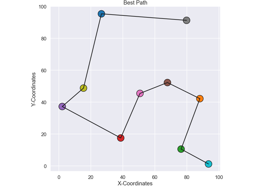
Ok, seems reasonable to me, problem solved I guess... Well, this brute force method will work fine for small problems where we do not have so many cities, like 10 in this case. The problem is that the number of permutations is given by the factorial of the number of cities, so for this specific case with 10 cities the total number of permutations is 10! = 3 628 800. If you instead had 15 cities the total number of permutations would be 15! = 1307 BILLIONS. Well, it seems fair to say that this brute force approach is not possible to use for a problem with just a bit more than 10 cities. Obviously we need to do something else so let’s look at a Genetic Algorithm (GA) to solve this problem!

The children of the (r)evolution

A genetic algorithm is inspired by the natural selection process and is a subgroup of evolutionary algorithms. A genetic algorithm is often used for optimization problems and relies on biologically inspired operators such as mutation, crossover and selection.

The first step is to generate an initial population where each individual is a possible solution to our problem. To be more specific, each individual within the population is an array which contains all numbers from 0 to 9 (we have 10 cities in this case).

Let’s write a helper function that generates an initial population.

def starting_population(nr_cities,population_size):
    
    population = np.array(np.zeros((population_size,nr_cities)),dtype=int)
    genome = np.arange(0,nr_cities)
    for i in range(0,population_size):
        np.random.shuffle(genome)
        population[i,:] = np.copy(np.array(genome,dtype=int))
    
    return population

Nice, now that we have a population of individuals it is time for nature to have its course to get the next generation of the population. Let’s summarize the different steps involved in this process.

Select parents.
Create a new individual by "crossing" the two parents.
Sometimes a mutation occurs...
Repeat until we have a new generation of the population
Elitism, the “best” solutions from the previous population are guaranteed to be included in the next generation

The steps above are then repeated a bunch of times and hopefully the population will be better and better for each generation. Let’s write some helper functions for the steps above and then put it all together to form our genetic algorithm.

But first, it is suggested from the steps above that we need to have some sort of measure of how "good" an individual is since we somehow are interested in the "best" solution. This will be done by a fitness function so let’s define this one first. We will use a very simple fitness function here that is given by one over the total traveled distance of the particular path. In code it looks like this:

def get_fitness(city_coords,population):
    
    fit = []
    for i in range(0,len(population)):
        
        fit.append( 1/total_distance(city_coords,population[i,:]) )
        
    return np.array(fit)

OK, not too complicated I guess. Now let’s look at each of the steps of the genetic algorithm.

Selecting parents

So, how to select two individuals from the current population to act as parents for a new individual of the next generation? Here we are loosely inspired by the phrase "Survival of the fittest" and the idea is that the individuals with a higher "fitness level" are more likely to be picked as parents. This is done by a bias roulette wheel method and the picture below shows in a schematic way how it works.

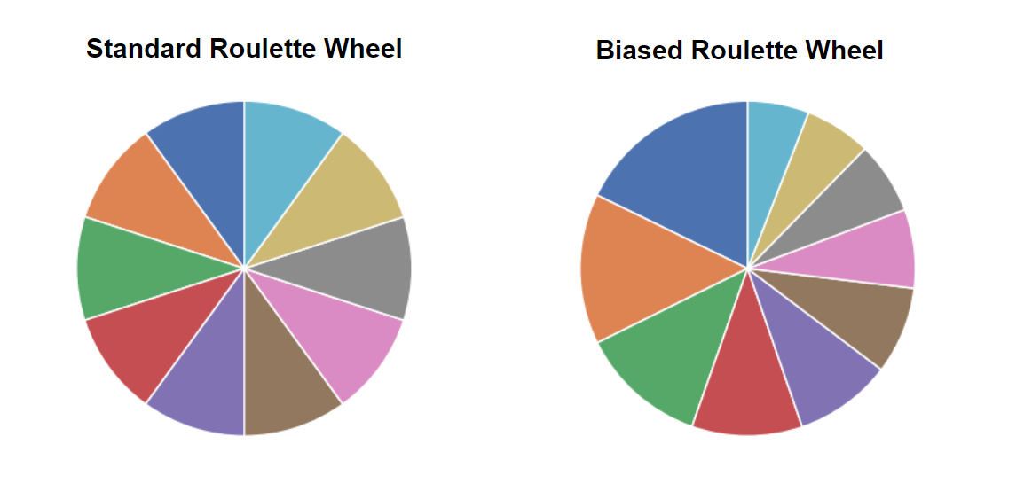
In a “standard” roulette wheel all numbers (in this case individuals of the population) have the same probability to occur but in a biased roulette wheel some numbers (individuals) are more likely to occur. To calculate this probability we simply use the fitness value of each individual and just normalize them by the sum of all fitness values. In code it looks like this

def select_parent(fit):
       
        probability = fit/np.sum(fit)
        parents_index = np.random.choice(np.arange(0,len(fit)),p=probability,replace=False,size=2)
        
        return parents_index

Note that in the numpy.random.choice function we have used replace=False just so we do not pick the same individual for both parents. Alright! Now we have two parents, let’s continue to the next function

Crossover

So, how do we mix the "DNA" or "genome" from both parents to become a new individual? Well, first of all, what is the genome for each individual? In this example it is simply the path i.e. a vector with all the numbers from 0 to 9 (for our current problem with 10 cities) with a certain order.

Now, how to do the actual mixing of the genome? One idea is just to split the genome from both parents and take the first part from the first parent and the second part from the second parent and then just put them together to form a new individual. Well, the problem with this is that each valid path (or genome) must contain all numbers from 0 to 9 (since it should visit all cities only once) and this can not be guaranteed by the procedure above.

So some modification is needed (but we are actually not that far away). What we need to do is something called ordered crossover and it goes something like this. Split the genome from parent 1 and keep the first part. For parent 2, remove all numbers found in the first part of parent 1 and keep the rest, with preserved order.

Ok, perhaps a bit cryptic but let’s write it in code.

def cross_over(genome_1,genome_2):
 
    index_split = np.random.randint(low=0,high=len(genome_1))
    
    head = genome_1[:index_split]
    tail = np.copy(genome_2)
    for i in head:
        tail = np.delete(tail,np.where(tail==i))
    
    child = np.zeros(len(genome_1))
    child[:index_split] = head
    child[index_split:] = tail
    
    return np.array(child,dtype=int)

Sweet! Now we have a child that is formed from the two parents but sometimes more things happen…

Mutation

Just as a flashback, mutation was a rather common feature in superhero comics back in the days

So, what would it mean in our example? First of all, the idea is that a mutation does not occur that often so we will have a parameter that controls the probability of a mutation happening. Moreover, in this blog post we are going to consider two different types of mutations called Mutation I and Mutation II (I know, not that catchy names...). In the first type of mutation we pick two numbers within the genome and simply just switch their location. For the second type of mutation we pick a location in the genome and then reverse the order of the first (or last) part of the genome. Let’s also write this in code.

def mutation(child):
    
    mutation = np.copy(child)
    if np.random.rand() > 0.5: # Mutation I
        
        switch_index = np.random.choice(np.arange(0,len(child)),replace=False,size=2)

        a = child[switch_index[0]]
        b = child[switch_index[1]]

        mutation[switch_index[0]] = b
        mutation[switch_index[1]] = a
        
        return mutation
      
    else:                      # Mutation II
        
        if np.random.rand() > 0.5:
            switch_index = np.random.randint(low=0,high=len(child))
            mutation[switch_index:] = np.flip(mutation[switch_index:])
        else:
            switch_index = np.random.randint(low=0,high=len(child))
            mutation[:switch_index] = np.flip(mutation[:switch_index])            
        
        return mutation

So, basically, what a mutation is doing is to give a different genome than the one obtained by crossing the genomes of the two parents and hopefully, as in the case of the superheros above, we can obtain a better one. It might be worse as well... we don’t know.

Elitism

Elitism is a way to ensure that the best individuals are carried over to the next generation. What we will do here is simply to include a predefined number of the best individuals in the next generation before we start with the procedure of populating the new generation by crossovers and mutations.

All together now (Life is Life)

So, It is now time to put it all together and see what kind of solution we would get. Here is the code:

population_size = 100
elite_size = 2
mutation_rate = 0.10
nr_gen = 200


best_fit_vector = []

# Get starting population
population = starting_population(nr_cities,population_size)
fit = get_fitness(city_coords,population)


for evos in range(0,nr_gen):


    next_gen = np.array(np.zeros(np.shape(population)),dtype=int)

    # keep the elite from previous population
    next_gen[:elite_size,:] = population[np.flip(np.argsort(fit))[0:elite_size],:]

    # populate next generation
    for i in range(elite_size,population_size):
    
        parents_index = select_parent(fit)
        child = cross_over(population[parents_index[0],:],population[parents_index[1],:])
        
        if np.random.rand() <= mutation_rate:
            child = mutation(child)
        
        next_gen[i,:] = child

    population = np.copy(next_gen)
    fit = get_fitness(city_coords,population)
    
    best_fit_index = np.where(fit[fit==np.max(fit)])[0][0]
    
    best_fit_vector.append(total_distance(city_coords,population[best_fit_index,:]))
    best_path_GA = population[best_fit_index,:]

We have stored the best path, i.e. the one with the highest fitness value from each generation. So let’s plot it and see how the best individual of the population changes as a function of the number of generations.

plt.figure(figsize=(8,6))
plt.plot(best_fit_vector)

plt.title('Best Distance = ' + str(np.round(best_fit_vector[-1],2)))

plt.xlabel('# generations')
plt.ylabel('Best Distance [-]')
plt.show()

and the plot

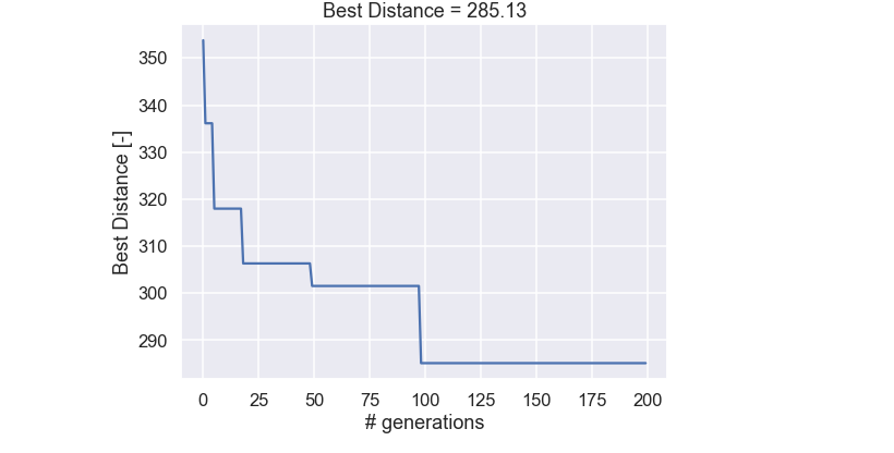
Ok, not to bad! There are some dramatic improvements in the beginning and as the solution gets better and better the improvement occurs more seldom. One more thing, Let’s plot the best path, obtained after 200 generations and see if this is the same as the brute force solution we did in the beginning of this blog post.

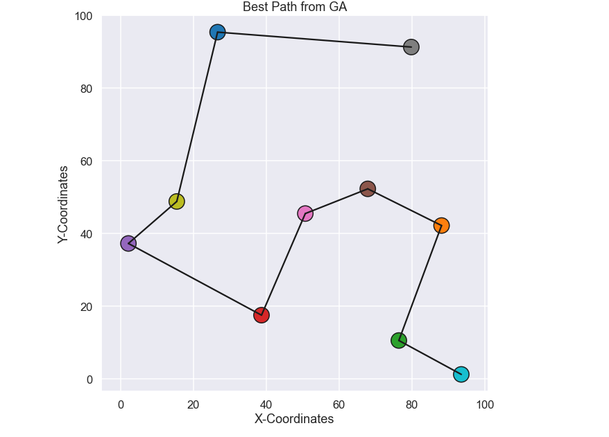
What do you know, it is the same path!! Bam! So it seems that our developed genetic algorithm gives promising results, let’s try it out on a larger problem!

More and More

It is time for the salesman to visit more cities, let’s try 25. By using the same code as above the following 25 cities have been generated.

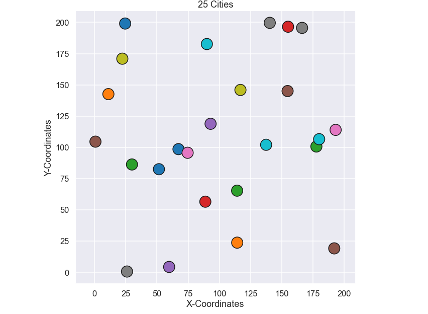
Just as a side note, if we were to try to solve this problem by a brute force method that was used in the very beginning of this post we would have to try 1.55e+25 permutations. That is a lot of permutations and if I were to run it on my computer it would take approximately 16000 BILLION YEARS i.e. 4000 times longer than the earth has existed! So, let’s not do that and instead run out genetic algorithm. We run the exact same code as for the example of 10 cities but with 1000 generations instead of 200.

OK, the run time was a lot faster than 16000 billion years. Let’s start by looking at the best individual for each generation.

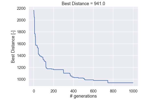
Nice! Similar behavior can be seen here, where the improvements are massive in the beginning but as more and more generations have been generated the improvements occur more seldom. Now we look at the best path from the initial (random) populations and compare it to the last generation.

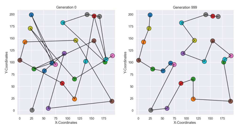
Ok, the path from the last generation seems much more logical to me at least, nice! Just as the last visualization I have included an animated gif with the best individual from each generation.

Time to conclude

So, we have implemented a genetic algorithm from scratch and even though the algorithm involves several concepts such as selection, cross over and mutations it was rather straightforward to implement.

I think there will be reasons to come back to a genetic algorithm in a future blog post since it is capable of solving really cool problems.

As always, feel free to contact us at info@gemello.se

A Genetic Algorithm

The Traveling Salesman problem