Alright, new blog post about optimization! In the last blog post about optimization we used a genetic algorithm to solve the classical traveling salesman problem. In this blog post we are going to use a similar algorithm to solve a multi-objective optimization problem (well, we are going to have two objective functions). This time we are “just” looking at some theoretical function but the ambition is to use this technique to solve a real world problem in an upcoming blog post. So let’s get started
You want it all but you can’t have it
For some reason I think about this song when multiobjective optimization is discussed
But let’s start to think about what it means to have more than one objective function, we are from now on assuming that we have two objective functions and we would like to minimize both of them. To make it even more concrete let’s look at an example
\[ \begin{split} f_1 & = 2\cdot x_1^2 + x_2^2 \\ f_2 & = (x_1 - 1)^2 + 2 \cdot (x_2 - 1)^2 \end{split} \]
and the constraints
\[ \begin{split} & -1.5 \leq x_1 \leq 1.5 \\ & -1.5 \leq x_2 \leq 1.5 \end{split} \]
So, here we can see the thing that often (well almost always) happens when you have more than one objective function, both objective functions are not minimized at the same time. In the example above \(f_1\) is minimized at \(x_1=0\) and \(x_2=0\) whereas \(f_2\) is minimized at \(x_1=1\) and \(x_2=1\). What to do then??
One way to deal with a multi objective optimization problem is to in some way combine the different objective functions into one single objective function, usually done by a weighted sum like
\[ f = w_1 \cdot f_1 + w_2 \cdot f_2 \]
After you have decided on the weights \(w_1\) and \(w_2\) you can use a single objective optimization algorithm to solve the problem. Well, this is where it, at least to me, gets a bit difficult. How should you choose the weights? Not that clear to me...
So let’s look at a different approach. Since we are (generally) not able to find a solution that minimizes both objective functions at the same time we are dealing with some sort of compromise. It would be really nice if we could find a set of solutions that represented “all the best” available solutions to the problem. Then, when we have “all the best” solutions we can choose the one we think is the best. By using this approach you somehow know what you are missing when you choose a specific solution. This was not the case for the situation above where you converted the problem from a multi-objective optimization problem since you had to choose the weights before knowing anything about the solution. So, let’s start to think about what we meen with “all the best” solutions and later on implement an algorithm for solving this.
Non-dominated solutions
Now, let’s look at the example given above. Since it "only" has two variables, \(x_1\) and \(x_2\), and two objective functions, \(f_1\) and \(f_2\), let’s look at "all" possible combinations of \(x_1\) and \(x_2\) see what is going on with \(f_1\) and \(f_2\). We do this by looking at a quite dense grid of \(x_1\) and \(x_2\) so let’s start with some python coding like the "standard" imports.
import numpy as np
import matplotlib.pyplot as plt
import pandas as pd

import seaborn as sns
sns.set(context='talk')
First we just define a function that takes a pandas dataframe as input that contains the variables \(x_1\) and \(x_2\) and returns a dataframe with the value of \(f_1\) and \(f_2\) added
def F_value(df_in):

    x1 = df_in['x1'].values
    x2 = df_in['x2'].values

    F1 = 2*x1**2 + x2**2
    F2 = (x1-1)**2 + 2*(x2-1)**2

    df_out = pd.DataFrame()

    df_out['x1'] = x1
    df_out['x2'] = x2

    df_out['f1'] = F1
    df_out['f2'] = F2

    return df_out
Now, let’s create a grid of \(x_1\) and \(x_2\) and for each pair calculate \(f_1\) and \(f_2\), then we make some nice looking plots.
X_low = [-1.5,-1.5]
X_high = [1.5,1.5]

x1_all = []
x2_all = []
for xx1 in np.linspace(X_low[0],X_high[0],500):
    for xx2 in np.linspace(X_low[1],X_high[1],500):
        x1_all.append(xx1)
        x2_all.append(xx2)


x1_all = np.array(x1_all)
x2_all = np.array(x2_all)

df_x_plot = pd.DataFrame()
df_x_plot['x1'] = x1_all
df_x_plot['x2'] = x2_all


df_plot = F_value(df_x_plot)


plt.figure(figsize=(16,7))

plt.subplot(1,2,1)
plt.scatter(x1_all,x2_all,c='lightgrey')

#plt.xlim(-2,2)
#plt.ylim(-2,2)
plt.xlabel('x_1')
plt.ylabel('x_2')
plt.title('Decision space')


plt.subplot(1,2,2)
plt.scatter(df_plot['f1'].values,df_plot['f2'].values,c='lightgrey')
plt.xlabel('F_1')
plt.ylabel('F_2')
plt.title('Objective space')


plt.show()
And the plots
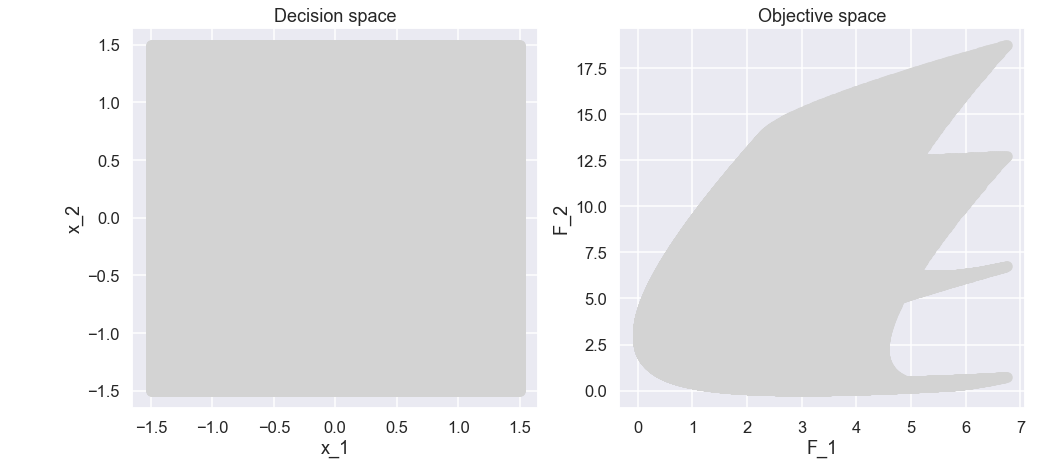
Ok, interesting. Since we would like to minimize both \(f_1\) and \(f_2\) let’s zoom in on the lower left part of the plot of the objective space.
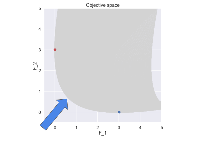
Here the minimum value of \(f_1\) and \(f_2\) have been marked. So, what solutions do you think comprises a good (the best) compromise between \(f_1\) and \(f_2\)? Well, apart from the two solutions that have been marked representing the individual minimums of \(f_1\) and \(f_2\), I would probably say the “”front” that is formed between the two marked solutions (marked with an arrow).
And why is that?
So, looking at any point on this front there is no solution that is better (smaller) in both \(f_1\) and\(f_2\) i.e. for any point on the front there is no other solution located further down and to the left, this is illustrated in the figure below.
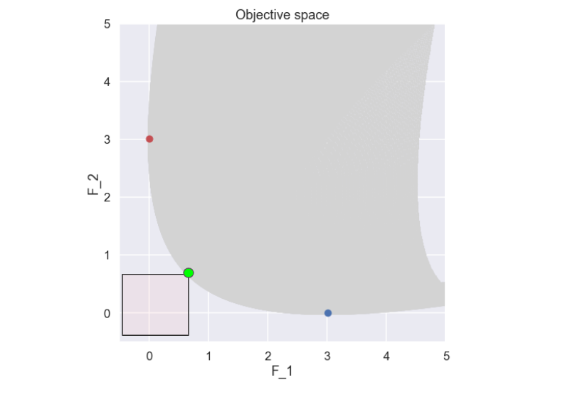
The solution marked by a green dot above is an example of a non-dominated solution as there is no other solution that is better in both \(f_1\) and \(f_2\) (i.e. there is no solution found in the semi transparent red box). To be a bit more precise, the definition of a non-dominated solution can be written as: A solution that cannot be improved in any of the objectives without degrading at least one of the other objectives
If you now collect all points that fulfill the criterias you have a non-dominated front. In this case where we have spanned the whole objective space (at least approximately) we know that is the best non-dominated front we can find and this is also referred to as a Pareto front.
So basically we are done now! We have now found the Pareto front which contains non-dominated solutions. Note that these different solutions on the pareto front are all considered equally good, so if we are to choose one specific solution some additional information has to be taken into consideration.
If we were to end here the blog post would be quite short, nothing wrong with that. But, it is obvious that not all problems can be solved by this brute force technique. If \(f_1\) and \(f_2\) were to be functions of several variables (like 7 or so) then the effort of spanning the whole design space would be huge.
So what to do instead?
NSGA-II
In the last blog post on optimization we used a genetic algorithm to solve a complicated problem so let’s try out a similar approach for our multi-objective optimization problem! The algorithm we are going to implement in python is similar to the famous NSGA-II algorithm which was originally developed by Deb et al. [1]. So, let’s start!
NSGA is short for Non-dominated Sorting Genetic Algorithm so in some way it is inspired by the nature where a population of individuals evolve during some time. To be a bit more specific the process can be described as:
We currently have a population of some size the following steps are taken in order to obtain the next generation
- Rank individuals in population
- Select a mating pool from the population
- Variation operator: get offspring
- Crossover
- Mutation
- Join current population and offspring together and rank the individuals
- Survivor operator: select individuals to be included in the next generation of the population
Note that when the above steps are taken we will have a new population of the same size as the original one. These steps are then repeated until some sort of termination criteria is fulfilled.
We will go through each individual step in detail later on but let’s start with the perhaps most important part. In any genetic algorithm we would like to give a ranking to each individual in the population. This is in order to give more emphasis on the individuals that are “good” and not promote the individuals that are “bad”. This is done in the selection of a mating pool, where the “good” individuals have a higher probability to be included in the mating pool, and the survival operator, where the “good” individuals are selected to be included in the next generation of the population.
So, what do we mean with “good” in our case of multi-objective optimization (remembering the stuff about Pareto front that we talked about in the beginning of the blog post)?
Well, there are actually two things that will determine if we think that a solution is “good” or “bad” and to understand them better we need to think about what we need in the end.
First of all, one of the end goals is that the individuals of the population should be located really close to the Pareto front, so somehow we have to promote the individuals that are closer to the Pareto front.
Secondly, we would like the individuals to be sort of equally spread over the Pareto front, so we do not want to end up with a bunch of individuals that are located more or less on the same spot.
So there will be two different measures that represent each of the two desired properties described above, the non-dominated sorting (or dominance depth) and the crowding distance. Let’s look at the one at the time!
Non-dominated sorting
So, let's look into the first of the two criteria that we use to rank each individual, this is done by a non-dominated sorting (this is quite central to the method... it is even in the name). This is perhaps best demonstrated by a small example. In the picture below we have 10 different solutions that make up a population (they are all marked with an individual number just to make the explanation a bit easier).
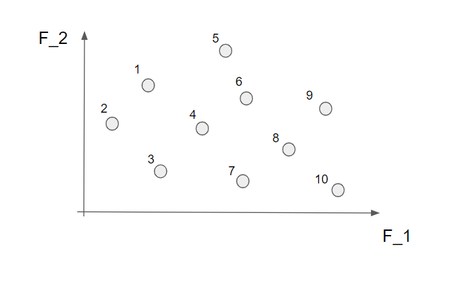
Now we start by identifying all the non-dominated solutions. Let's start with the first solution (nr 1). To find out if this is a non-dominated solution or not we simply look to the left and below this point to figure out if there are any solutions in this area.
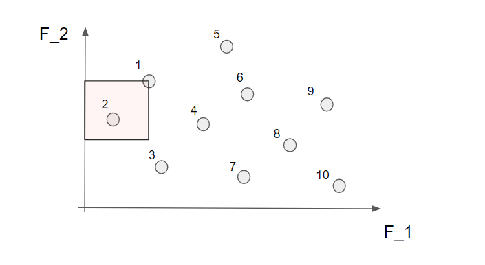
Well, we see that nr 2 can be found in this area so the solution nr 1 is not a non-dominated solution. Let's continue to the next solution (nr 2).
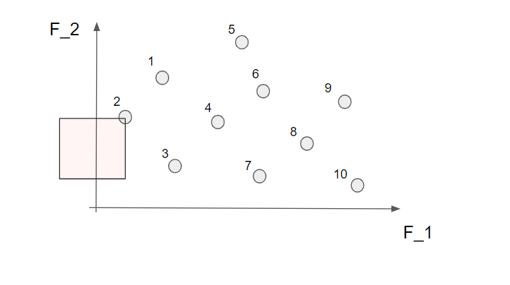
Here we can not find any other solution in the marked area so this is indeed a non-dominated solution! Alright! If we continue to do this for all the 10 solutions we find that nr 2, 3, 7 and 10 are non-dominated solutions.
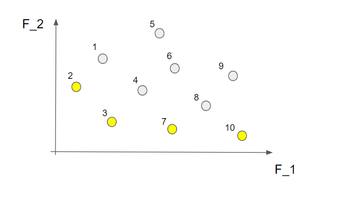
This is called the first non-dominated front and contains the "best" solutions from this perspective. What we do now is to temporarily disregard the solutions from the first non-dominated front and do the same procedure all over again. This time we find the following non-dominated solutions marked in brown in the picture below (the solutions from the first non-dominated front are still marked in yellow)
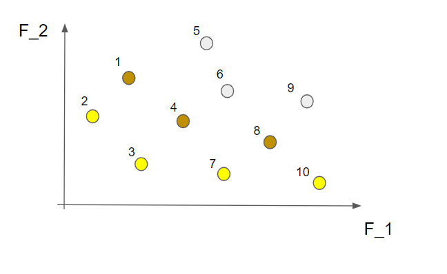
These solutions make up the second non-dominated front. If we now temporarily forget about these solutions, as well as the ones in the first non-dominated front, and repeat the same steps as above we will have the third non-dominated front. Like this
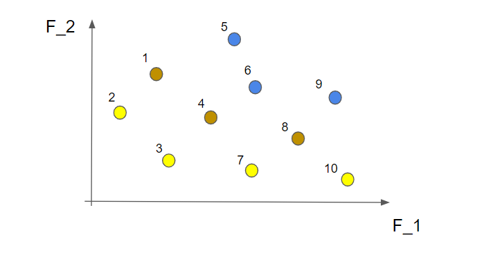
OK, we have now sorted all the different solutions into a number of non-dominated fronts. Just to clarify, the solutions within a front are all considered equal as good but the solutions in the first non-dominated front are better than the solutions in the second non-dominated front. So, we are now ready to write a small function that takes the dataframe that contains the \(x_1\) and \(x_2\) variables as well as the two objective functions \(f_1\) and \(f_2\) as inputs and returns a dataframe that also contains a number for each solution that represents which non-dominated front it belongs to.
def find_non_dominated_fronts(df_in,population_size):

    F1 = df_in['f1'].values
    F2 = df_in['f2'].values

    x1 = df_in['x1'].values
    x2 = df_in['x2'].values


    front_index = []
    F1_fronts = []
    F2_fronts = []
    x1_fronts = []
    x2_fronts = []

    # Find non-dominated fronts

    for j in range(1,25):
        dominated_index = []

        for ii in range(0,len(F1)):

            if np.sum((F1<F1[ii]) & (F2<F2[ii]) ) == 0:
                dominated_index.append(ii)

                F1_fronts.append(F1[ii])
                F2_fronts.append(F2[ii])
                x1_fronts.append(x1[ii])
                x2_fronts.append(x2[ii])
                front_index.append(j)

        F1[dominated_index] = 1000
        F2[dominated_index] = 1000

        if len(front_index)>=population_size:
            break

    df_out = pd.DataFrame()
    df_out['x1'] = x1_fronts
    df_out['x2'] = x2_fronts
    df_out['f1'] = F1_fronts
    df_out['f2'] = F2_fronts
    df_out['front_nr'] = front_index

    return df_out
Alright! We have now covered a realy central part of this algorithm, let's look into some stuff that is related to the second criterion i.e. the divercity
Crowding distance
So, since we ultimately would like to have the individuals in the population spread out rather evenly over the Pareto front we need to have some measurement of how close the solutions are to each other (in the objective space). There are of course several ways to measure this and we are going to use the crowding distance. We will also demonstrate this by a small example with the solutions below.
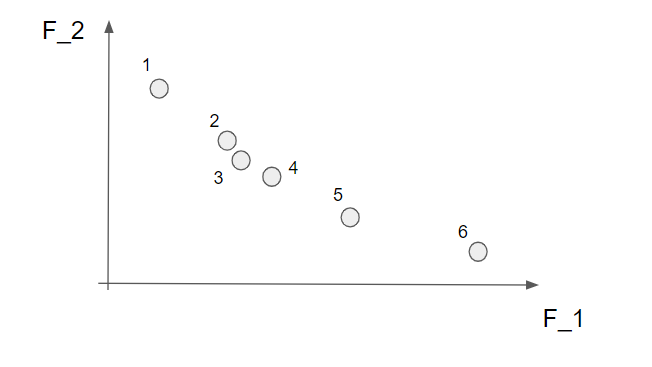
Note that the crowding distance is calculated within each non-dominated front so this needs to be calculated prior to the calculation of the crowding distance. Already here we can say that solutions 2, 3 and 4 are close to each other and perhaps we do not need all these solutions since they give approximately the same information.
Now we start with the first objective function, \(f_1\) and sort the solutions according to their \(f_1\) values. Here we are “lucky” since the points are already sorted from the smallest to the largest but, generally, the first step is to sort the solutions in the first objective function. Now, the solutions with the largest and the smallest value we would like to keep since they describe the most extreme solutions within the front. These end values are automatically assigned a really high number.
For the other solutions we calculate the distance between the solution to the right of the current solution and to the left of the current solution and divide it by the distance between the largest and smallest solutions. Perhaps an example. Looking at the solution nr 2 (makred in red below) we calculate the crowding distance by the distance between solution 3 and solution 1 divided by the distance between solution 6 and solution 1.
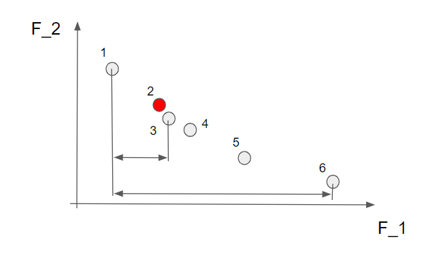
Nice! Just note here that the crowding distance for solution 3 is really small compared to the other solutions since both solution 4 and 2 are close by.
When we have calculated the distance in the first objective function we do the exact same thing for the second objective function \(f_2\). When this is done we get the total crowding distance by just adding the distances for \(f_1\) and \(f_2\).
Now, let’s do some more coding.
def crowding_distance(df_fronts):

    unique_fronts = np.unique(df_fronts['front_nr'].values)

    df_crowding_distance = pd.DataFrame()
    for ii in range(0,len(unique_fronts)):
        df_temp = df_fronts[df_fronts['front_nr']==unique_fronts[ii]]

        # --- sort by f1
        df_temp_f1 = df_temp.sort_values('f1')

        cd_1 = np.zeros(len(df_temp_f1))
        f1_values = df_temp_f1['f1'].values

        cd_1[0]  = 10000
        cd_1[-1] = 10000

        for i in range(1,len(cd_1)-1):
            cd_1[i]= (f1_values[i+1]- f1_values[i-1]) / (f1_values[-1]-f1_values[0])

        df_temp_f1['cd_1'] = cd_1

        # --- sort by f2
        df_temp_f2 = df_temp_f1.sort_values('f2')

        cd_2 = np.zeros(len(df_temp_f2))
        f2_values = df_temp_f2['f2'].values

        cd_2[0]  = 10000
        cd_2[-1] = 10000

        for i in range(1,len(cd_2)-1):

            cd_2[i]= (f2_values[i+1]- f2_values[i-1]) / (f2_values[-1]-f2_values[0])

        df_temp_f2['cd_2'] = cd_2

        # --- calculate total distance
        df_temp_f2['cd_total'] = df_temp_f2['cd_1'] + df_temp_f2['cd_2']

        df_crowding_distance = pd.concat([df_crowding_distance,df_temp_f2])


    df_crowding_distance_sorted = df_crowding_distance.sort_values(['front_nr','cd_total'],ascending=[True,False])

    return df_crowding_distance_sorted
So the dataframe now contains information about both which non-dominated front each solution belongs to and the crowding distance. For later purposes we have also sorted the dataframe first on the non-dominated front number and then on crowding distance.
Sweet! Now we have covered two of the most important things for the NSGA-II, the non-dominated sorting and crowding distance. So, let’s go back to the different steps that are involved in the algorithm (assuming we have a current population of a predefined size).
- Rank individuals in population
- Select a mating pool from the population
- Variation operator: get offspring
- Crossover
- Mutation
- Join current population and offspring together and rank the individuals
- Survivor operator: select individuals to be included in the next generation of the population
The ranking thing we have sort of already done in the sense that we know how to do the non-dominated sorting, so every individual belongs to a certain front, and how to calculate the crowding distance for each individual. So let’s look at the remaining steps one by one!
Select a mating pool from the population
So here we select the individuals that will be used as parents for the next generation of the population. As already touched upon, we would like to promote the “good” individuals so they have a higher representation in the matting pool. So how do we do this then? There are several options but here we are going to use the binomial tournament selection.

The idea is quite simple, you pick two individuals from the population, they have a “fight” and the best one wins a place in the mating pool. How do you then win a fight? The individual who belongs to the best non-dominated front (low number) will always win over the opponent so this is the first thing to check. If both individuals belong to the same non-dominated front the one with the best crowding distance (larger is better) will win. In the case where both individuals belong to the same non-dominated front and have the same crowding distance the winner will be decided by flipping a fair coin.
One more thing, the selection of which individuals that are to “fight” is done without replacement so each individual will participate in one fight. So if the population size is 30 we will have 15 winners that are selected for the mating pool and since we would like the mating pool to have the same size as the population size we have to run two tournaments. I think we are ready to write some more code now!
def binomial_tournament_selection(df_crowding_distance):

    idx = np.arange(0,len(df_crowding_distance))
    winner_idx = []

    for ii in range(0,2):

        np.random.shuffle(idx)

        for jj in np.arange(0,len(idx)-1,2):

            idx_1 = idx[jj]
            idx_2 = idx[jj+1]


            f1  = df_crowding_distance.iloc[idx_1,4]
            f2  = df_crowding_distance.iloc[idx_2,4]
            cd1 = df_crowding_distance.iloc[idx_1,-1]
            cd2 = df_crowding_distance.iloc[idx_2,-1]


            if f1<f2:
                winner_idx.append(idx_1)
            if f2<f1:
                winner_idx.append(idx_2)
            if f1==f2:
                if cd1>cd2:
                    winner_idx.append(idx_1)
                if cd2>cd1:
                    winner_idx.append(idx_2)
                if cd1==cd2:
                    if np.random.rand()<0.5:
                        winner_idx.append(idx_1)
                    else:
                        winner_idx.append(idx_2)


    df_mating_pool =  df_crowding_distance.iloc[winner_idx,:2]


    return df_mating_pool
Crossover and mutation
Now we have a mating pool that we can select parents from so the next thing to decide on is how do we combine two parents to create offspring. Here we are using something called Simulated Binary Crossover (SBX) which we should spend some time on now. You can also check out the paper by Deb and Agrawal [2]
Note that both crossover and mutation are done in the decision space or, in this case, the \(x_1\) and \(x_2\) variables. Moreover crossover is done for one \(x\) variable at a time
First of all this method takes two parent individuals as input, \(P_i^1\) and \(P_i^2\), and creates two offspring individuals, \(O_i^1\) and \(O_i^2\). The two offstring are defined as
\[ \begin{split} O_i^1 & = 0.5 \cdot [ P_i^1 (1-\beta_i) + P_i^2 (1+\beta_i) ] \\ O_i^2 & = 0.5 \cdot [ P_i^1 (1+\beta_i) + P_i^2 (1-\beta_i)] \end{split} \]
One of the properties of SBX is that the offspring have the same mean value as the parents i.e. \( 0.5(O_i^1+O_i^2) = 0.5(P_i^1+P_i^1) \), a property that is found for binary crossover. Moreover, we need to define the \(\beta_i\) parameter. \(\beta_i\) will describe the relation between the spread of the offspring in relation to spread of the parents, defined as
\[ \beta_i = \frac{|O_i^2-O_i^1|}{|P_i^2-P_i^1|} \]
So a \(\beta < 1\) means that the spread of the offspring is smaller than the spread of the parents. One more thing, it is assumed that \(P_i^2 > P_i^1\) and if this is not true you simply switch place of \(P_i^1\) and \(P_i^2\).
So how do we get \(\beta_i\)? The authors of the paper suggested a probability function of \(\beta_i\) according to:
\[ p(\beta_i) = \begin{cases} 0.5(\eta_c + 1)\beta_i^{\eta_c}, &\beta_i \leq 1\\ 0.5(\eta_c + 1)\frac{1}{\beta_i^{\eta_c+2}}, &\text{otherwise} \end{cases} \]
Below is a plot of the function
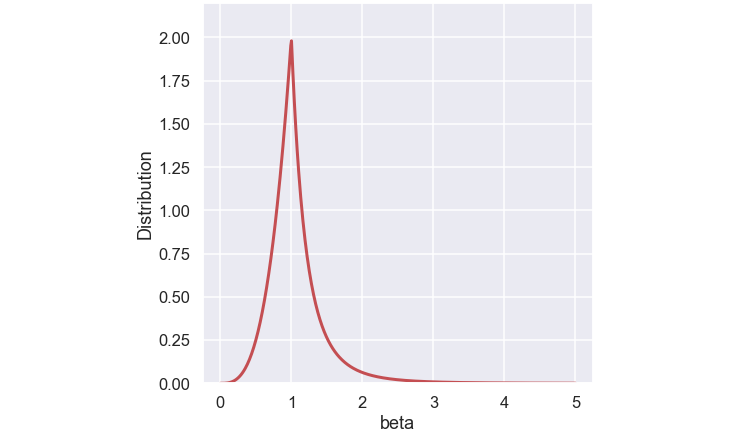
The \( \eta_c \) is the SBX crossover operator distribution factor that is a user defined parameter. Below is a plot of the function for some different values of \(\eta_c\)
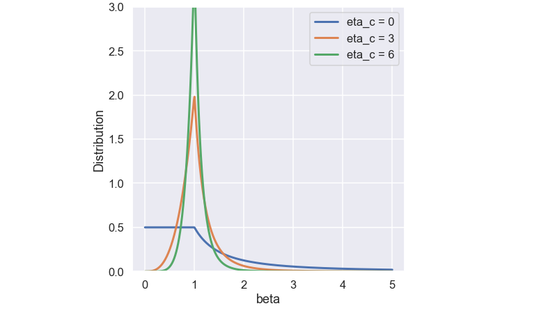
The function is constructed so the total area below the curve is one (since it is a probability function).
The procedure of finding the \(\beta_i\) value is to draw a random number, \( u_i\), between 0 and 1 and then find the \(\beta_i\) where the area under the curve corresponds to \(u_i\), see the picture below.
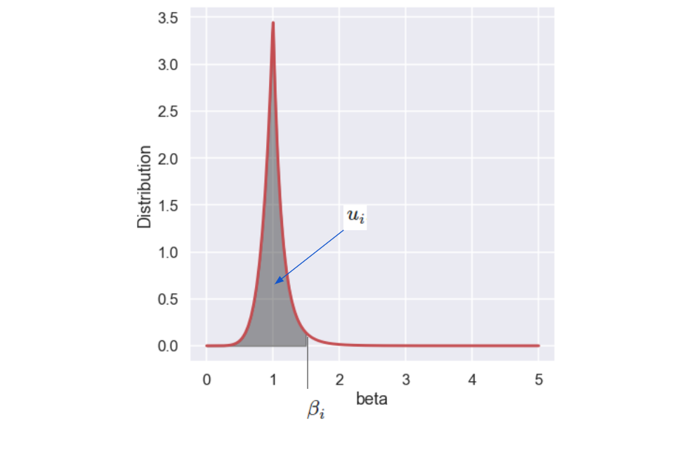
Luckily, there is a closed form expression for \(\beta_i\) as a function of \(u_i\) given by:
\[ \beta_i = \begin{cases} 2(u_i)^{\frac{1}{\eta_c + 1}}, &u_i \leq 0.5\\ (\frac{1}{2(1-u_i)})^{\frac{1}{\eta_c + 1}}, &\text{otherwise} \end{cases} \]
Nice, let’s write a function that does the crossover as discussed above!
def SBX(P1,P2,eta_c):


    O1 = np.zeros(len(P1))
    O2 = np.zeros(len(P1))

    for ii in range(0,len(P1)):

        if P1[ii]<P2[ii]:
            p1 = P1[ii]
            p2 = P2[ii]
        else:
            p1 = P2[ii]
            p2 = P1[ii]

        u_i = np.random.rand()
        if u_i<=0.5:
            beta_i = (2*u_i)**(1/(eta_c+1))
        else:
            beta_i =1 / ( (2*(1-u_i))**(1/(eta_c+1)))

        o1 = 0.5*( (1-beta_i)*p1 + (1+beta_i)*p2 )
        o2 = 0.5*( (1+beta_i)*p1 + (1-beta_i)*p2 )

        O1[ii] = o1
        O2[ii] = o2

    return O1,O2
So now when we have created offspring according to the SBX method we can add to the variation by using a mutation operator. Mutations are something that is quite rare so we need to define a mutation rate (typically in the range of a few percent). In the case where a mutation takes place we are using a method called Polynomial Mutation Operator. The mutation is described by
\[y_i = x_i + \delta_i(x_i^U - x_i^L) \]
where \(x_i\) is the value before mutation and \(y_i\) is the value after mutation.
So, similarly to the crossover operator we do the mutation for one variable at the time. Since the upper and lower bound of the variable are known we “only” need to define the \(\delta_i\) value. Similar to the crossover operator we define probability function as
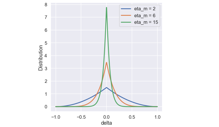
\[ p(\delta_i) = 0.5(\eta_m + 1)(1-|\delta_i|)^{\eta_m} \]
A plot of the probability function is found below
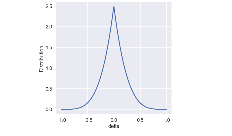
Similar to the SBX function the \( \eta_m\) is a user defined variable that controls the shape of the function. A plot of the function for some different values of \( \eta_m\) is shown below.
Just as above we find the value of \(\delta_i\) by generating a random number \(r_i \in [0,1] \) and this time use the following closed form:
\[ \delta_i = \begin{cases} (2 r_i)^{\frac{1}{\eta_m + 1}}, &r_i \le 0.5\\ 1 - [2(1-r_i)]^{\frac{1}{\eta_m + 1}}, &r_i \geq 0.5 \end{cases} \]
It is once again coding time
def mutation(O,eta_m,propability_mutation,X_low,X_high):


    if np.random.rand()<propability_mutation:

        O_mutation = np.zeros(len(O))

        for ii in range(0,len(O)):

            o = O[ii]

            r_i = np.random.rand()
            exp_factor = 1/(eta_m+1)

            if r_i < 0.5:
                delta_i = (2*r_i)**exp_factor - 1
            else:
                delta_i = 1 + (2*(1-r_i))**exp_factor

            o_mutation = o + (X_high[ii]-X_low[ii])*delta_i

            O_mutation[ii] = o_mutation


    else:
        O_mutation = np.copy(O)

    return O_mutation
Nice! We have now looked at how to combine two parent individuals into two new individuals, so we are almost done!
What we do next is to randomly take out two parents from the mating pool and by the help of crossover and mutation form two offspring individuals. This we do several times until we have a population of offspring individuals that have the same size as the current population
Let’s continue with the survivor operator
Survivor operator
So, the job of the survivor operator is to determine which individuals will make it to the next generation of the populations. As touched upon previously we want the individuals that are “good” to be included and the “not so good” to be excluded. Before we have a look at how the survivor operator works let’s review what we have so far. At the moment we have a current population of a predefined size. We also have a set of offspring individuals with the same size as the current population. What we do now is to smash these two populations together and form a set of individuals with double the population size. This large population is then ranked according to the non-dominated fronts and crowding distance. Now start the job of the survivor operator to find the individuals that will be included in the next generation. This next generation must be of the same size as the current population so half of the ranked individuals will not make it. So how is this then done? To start with let’s look at the picture below
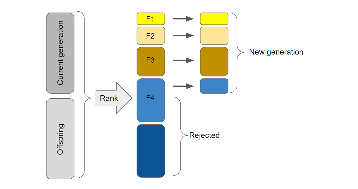
We know that the next generation of the population must have the same size as the current population so we start by looking at all the individuals that belong to the first non-dominated front and see if they all fit into the new generation, well perhaps they do. Let’s continue to look at the individuals that belong to the second non-dominated front, will they also fit into the next generation? Let’s assume they do. Same with the members of the third front. Now, when we look at the members of the fourth non-dominated front, there is not room for all of them in the next generation since then the next generation will be larger than the current population. So we must look at something else in order to find out members of the fourth non-dominated front that will be included in the next generation. This is where the crowding distance comes into the picture to discriminate the members within a front.
Yes I know, a lot of text but in the end it seems quite simple. Start to include individuals into the next generation based on their non-dominated front ranking and if not all members fit into the next generation use the crowding distance.
Let’s try it out!
Man, this is a long blog post but we are almost there! The last thing is to put it all together and make a test run. Since we have discussed a lot of things, let's just remember what the end goal is. We start with an initial population of a predefined size. The idea is then that the individuals of the population will end up near the complete Pareto front as we run the genetic algorithm for several generations. OK, let’s write some code that puts it all together.
population_size = 60
eta_c = 15

propability_mutation = 0.05
eta_m = 20

# -------------- for plotting ------------

X1_plot = []
X2_plot = []
F1_plot = []
F2_plot = []
Front_plot = []


# ------- initial population ------------
x1_population = np.random.uniform(X_low[0],X_high[0],size=population_size)
x2_population = np.random.uniform(X_low[1],X_high[1],size=population_size)

df_x = pd.DataFrame()
df_x['x1'] = x1_population
df_x['x2'] = x2_population

df_f = F_value(df_x)


# sort by non dominated fronts
df_fronts = find_non_dominated_fronts(df_f,population_size)

# crouding distance
df_survival = crowding_distance(df_fronts)


# -------------- for plotting ------------
X1_plot.append(df_survival.x1.values)
X2_plot.append(df_survival.x2.values)
F1_plot.append(df_survival.f1.values)
F2_plot.append(df_survival.f2.values)
Front_plot.append(df_survival.front_nr.values)


for nr_gen in range(0,201):

    # --- mating pool
    mating_pool = binomial_tournament_selection(df_survival)

    # --- crossover and mutation
    O_x1 = []
    O_x2 = []

    idx_crossover = np.arange(0,population_size)
    np.random.shuffle(idx_crossover)

    for jj in np.arange(0,len(idx_crossover)-1,2):
        idx_1 = idx_crossover[jj]
        idx_2 = idx_crossover[jj+1]
        P1    = mating_pool.iloc[idx_1,:].values
        P2    = mating_pool.iloc[idx_2,:].values


        O1,O2 = SBX(P1,P2,eta_c)
        O1_mutated = mutation(O1,eta_m,propability_mutation,X_low,X_high)
        O2_mutated = mutation(O2,eta_m,propability_mutation,X_low,X_high)

        O_x1.append(O1_mutated[0])
        O_x1.append(O2_mutated[0])

        O_x2.append(O1_mutated[1])
        O_x2.append(O2_mutated[1])


    df_offspring = pd.DataFrame()

    df_offspring['x1'] = O_x1
    df_offspring['x2'] = O_x2

    df_x_all = pd.concat([df_survival.iloc[:,:2],df_offspring])
    df_f = F_value(df_x_all)

    # --- Constraints
    idx_constraint_violation_x1 = np.where(np.logical_or(df_f.x1 < X_low[0], df_f.x1 > X_high[0]))[0]
    idx_constraint_violation_x2 = np.where(np.logical_or(df_f.x2 < X_low[1], df_f.x2 > X_high[1]))[0]

    if len(idx_constraint_violation_x1) > 0:
        for i in idx_constraint_violation_x1:
            df_f.iloc[i,2] = 1e6
            df_f.iloc[i,3] = 1e6

    if len(idx_constraint_violation_x2) > 0:
        for i in idx_constraint_violation_x2:
            df_f.iloc[i,2] = 1e6
            df_f.iloc[i,3] = 1e6

    # sort by non dominated fronts
    df_fronts = find_non_dominated_fronts(df_f,population_size)

    # crowding distance
    df_crowding_distance = crowding_distance(df_fronts)

    # Survival
    df_survival = df_crowding_distance.iloc[0:population_size,:]

    # ----- Store for plotting ---------
    X1_plot.append(df_survival.x1.values)
    X2_plot.append(df_survival.x2.values)
    F1_plot.append(df_survival.f1.values)
    F2_plot.append(df_survival.f2.values)
    Front_plot.append(df_survival.front_nr.values)
Sweet! Note that we have included a very simple way to handle the constraints of the design space. If an individual is located outside of the allowed region, the objective functions will automatically get a really high value.
To start with, why not have a look at the initial population in both design space and objective space, note that all individuals are generated randomly. Here we also have included all solutions in the background just for reference.
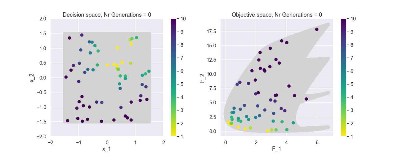
The color represents the non-dominated front number. Now, let’s have a look at the population after 200 generations.
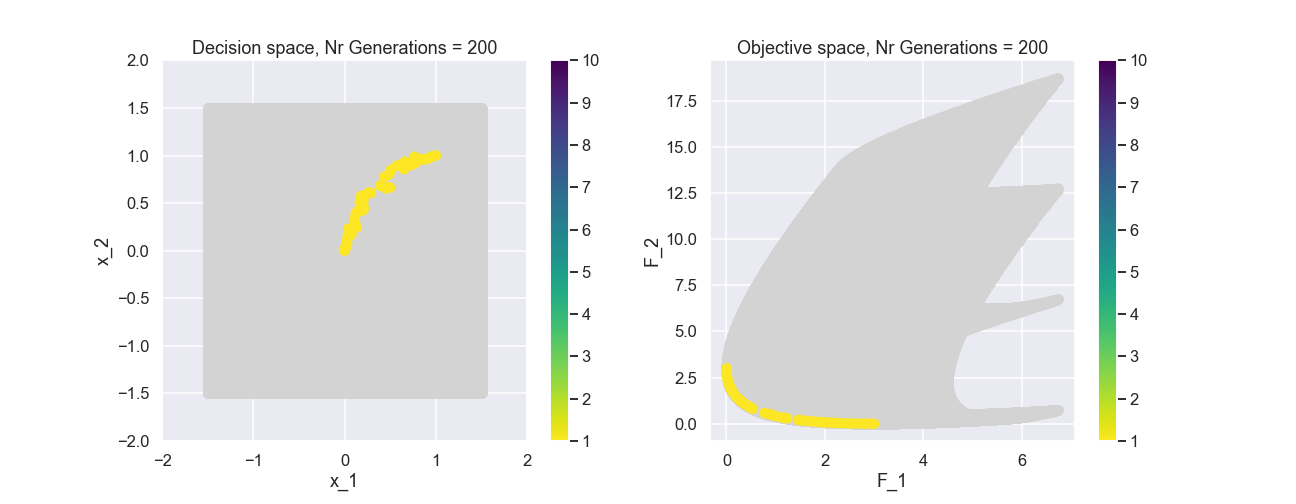
This actually looks quite nice! The individuals of the population are fairly evenly spread out and near the true Pareto front.
As a last visualization let’s include an animated gif that contains a bunch of generations of the population.
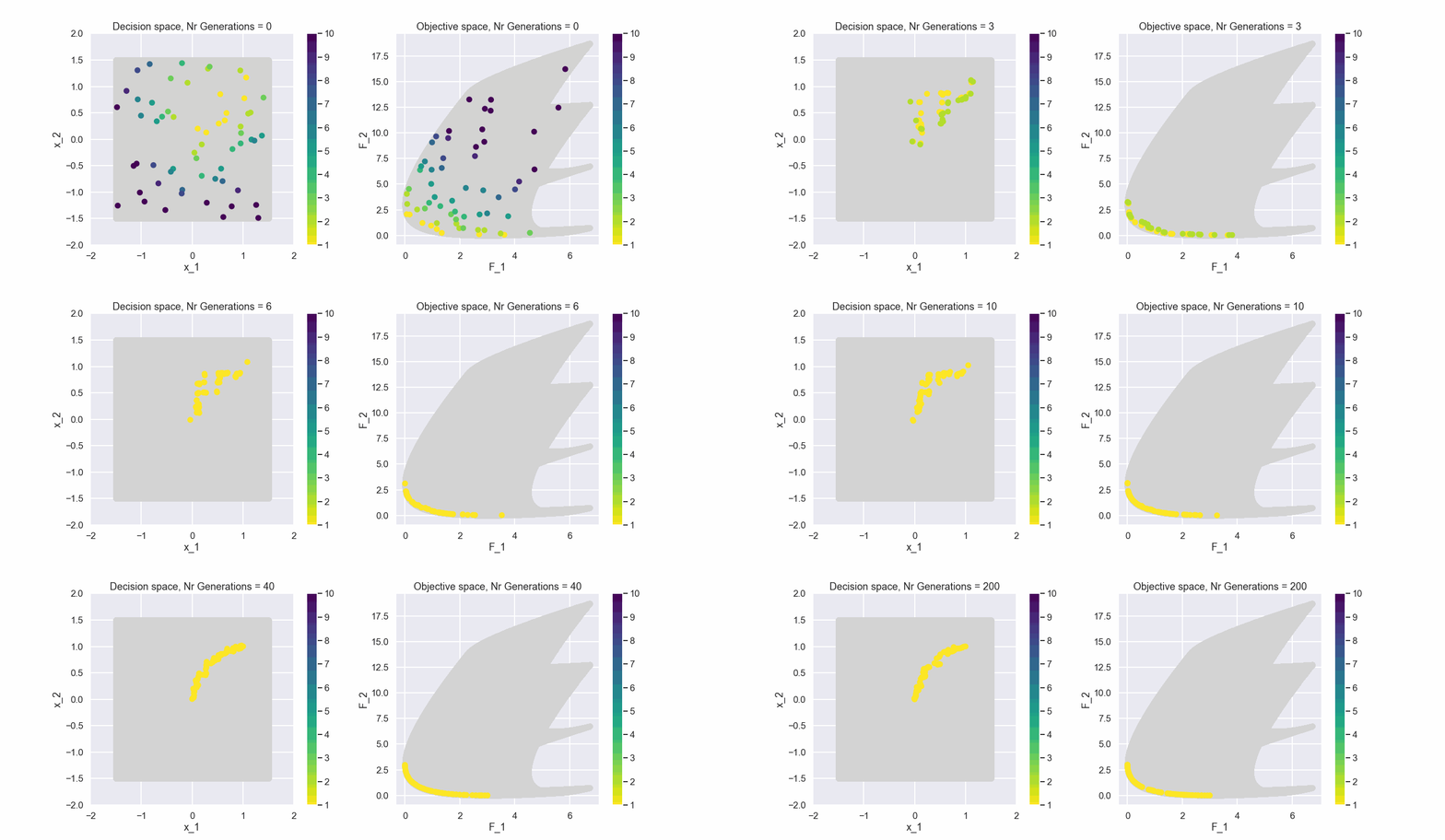
What can be seen is that after just a few generations most of the individuals in the populations belong to the first non-dominated front.
Time to conclude
As mentioned before, this was a really long blog post! The reason for this is that quite many new concepts had to be covered.
I think that the most important thing to take away is that when you deal with multi-objective optimization the end result is not one optimal solution. In this example where we had two objective functions the non-dominated front was a line. If we had three objective functions the non-dominated front would be a surface.
We also had a shot at implementing something similar to the NSGA-II algorithm where the concepts of non-dominated sorting and crowding distance were explained.
Well I guess that was all for this time and, as always, feel free to contact us at info@gemello.seReference
[1] K. Deb, A. Pratap, S. Agarwal and T. Meyarivan, "A fast and elitist multiobjective genetic algorithm: NSGA-II," in IEEE Transactions on Evolutionary Computation, vol. 6, no. 2, pp. 182-197, April 2002, doi: 10.1109/4235.996017.
[2] K. Deb and R.B Agarwal, "Simulated Binary Crossover for Continuous Search Space," Complex Systems, vol. 9, no. 2, pp. 115-148, 1995.