Time for a new blog post on optimization! In these two previous blog posts on optimization (here and here) we looked at some nature inspired optimization techniques that could be sorted under genetic algorithms. In this blog post we are going to look at a different optimization technique that is inspired by nature, a particle swarm optimization algorithm. As it turns out, this is actually a fairly simple algorithm to implement and we will do this from scratch in python (of course!)
I want problems
In this blog post we are not going to solve a “real world” problem (maybe in a later blog post) instead we are going to look at the minimization of the Rosenbrock function, more specifically the 2-dimensional version given by:
\[ f(x_1,x_2) = (1-x_1)^2 + 100 \cdot (x_1 - x_2^2)^2 \]
and the constraints
\[ \begin{split} & -5 \leq x_1 \leq 5 \\ & -5 \leq x_2 \leq 5 \end{split} \]
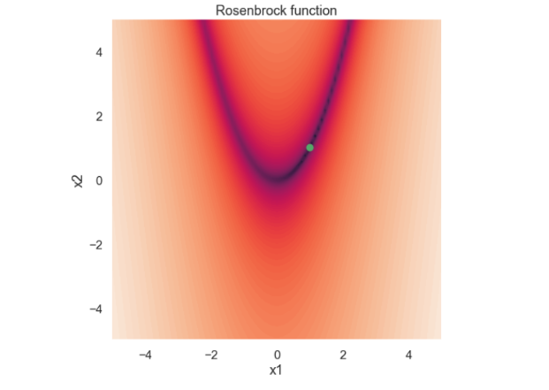
By inspecting the function above it is clear that the global minimum of the function is located at \( (x_1,x_2) = (1,1) \). Below is a visualization of the Rosenbrock function, \( ln(f) \), where the global minimum is marked.

If you would like to read more about the Rosenbrock function you can, for instance, have a look at the Wikipedia site.
Everybody's heard about the bird
So what is this particle swarm optimization all about then? As the name suggests there is a swarm of particles involved and each particle is characterized primarily by its coordinate. In one way it is similar to the genetic algorithms that was investigated in the previous blog post since we start with a “population” of individuals of a certain predefined size. However, for the genetic algorithm we obtained new generations of the population by crossing over or mating between the different individuals. This doesn't happen in a particle swarm optimization algorithm where the location of each individual is updated in some (randomized) manner. So, basically, we “only” need a method that calculates the velocity for each particle for each instance of time and then we are done! Let’s start with that.
Just before we start to look into the actual equations of the velocity it can be useful to think of the particle swarm as a flock of birds that is searching for food. The flock is made up of individual birds that will have their own personal experience about where the best location to find food is. Moreover, you can also think that somehow the birds are looking for food in a collective way so if one bird finds a really nice place it will tell the other birds in the flock.
So, the velocity of each particle (or bird) is made up of three different parts
\[ \boldsymbol{v}_i^{t+1} = w \cdot \boldsymbol{v}_i^{t} + c_1 \cdot r_1 \cdot (\boldsymbol{x}_{b,i} - \boldsymbol{x}_i^{t}) + c_2 \cdot r_2 \cdot (\boldsymbol{x}_{g} - \boldsymbol{x}_i^{t})\]
Let’s try to understand them one at a time.
The first term, \(w \cdot \boldsymbol{v}_i^{t} \), is referred to as the momentum part where \(\boldsymbol{v}_i^{t} \) is the velocity from the previous time step. This part represents inertia in some way as it just says that a particle will continue to move in the direction that it already has.
The second term, \( c_1 \cdot r_1 \cdot (\boldsymbol{x}_{b,i} - \boldsymbol{x}_i^{t}) \), is the cognitive part. The idea behind the cognitive part is that each particle (or bird) has a memory of the best location it has ever visited. This location is stored in the \( \boldsymbol{x}_{b,i} \) vector so the term \( (\boldsymbol{x}_{b,i} - \boldsymbol{x}_i^{t}) \) is a vector that directs each particle towards its, so far, best location. Sort of like nostalgia! Moreover, the \(r_1\) is a random number between 0 and 1 and \(c_1\) is a constant
Finally, the third term, \( c_2 \cdot r_2 \cdot (\boldsymbol{x}_{g} - \boldsymbol{x}_i^{t}) \) ,is called the social part. Here \( \boldsymbol{x}_{g} \) is the best location any particle (or bird) has visited so it represents the best location of the swarm. As a consequence, the term \( ( \boldsymbol{x}_{g} - \boldsymbol{x}_i^{t}) \) will direct each particle towards the current best position known to the particle swarm. The analogy to the flock of birds would be that somehow the birds communicate with each other and reveal the best location they have found. Similar to the cognitive part the term \(r_2\) is a random number between 0 and 1 and \(c_2\) is a constant.
OK! That was more or less it! After we have calculated the velocity of each particle we just update the location of each particle according to
\[ \boldsymbol{x}_i^{t+1} = \boldsymbol{x}_i^{t} + \boldsymbol{v}_i^{t+1} \]
(Here it is assumed that one time unit has elapsed during the update and that is why we don't see a \( \Delta t \) in the equation above )
Boom, or as Manolo golf would say:

Some more things before we start with the coding. As stated above we have some constraints on both \(x_1\) and \(x_2\) and we must somehow make sure that we are inside the allowed region of the search space. How to do this? Well, let’s just do the simplest thing possible! if a particle is outside the allowed area we just project it back to the boundary. Allow me to do demonstration! (also an expression from Manolo golf :-) ) If a particle gets a new position of \( (x_1,x_2) = (6.2,3.9) \) where \(x_1\) is outside the allowed region we just project it back to the boundary so the new position would be \( (x_1,x_2) = (5.0,3.9)\).
The initiation of variables we also need to look at. The initial position of each particle is assigned by just picking two random numbers within the allowed region. Moreover, the initial velocity is set to zero for each particle.
So, I think that we are finally ready to do some coding!
First, the usual imports
import numpy as np
import matplotlib.pyplot as plt
import seaborn as sns

sns.set(context='talk')
We need a function that evaluates the function that is to be optimized
def func_eval(x1,x2):

    f = (1-x1)**2 + 100*(x2-x1**2)**2

    return f
And now, here is the main program
population_size=50

w_max = 0.9
w_min = 0.1
c1 = 1.5
c2 = 1.5
t_max = 50

x1_min = -5
x1_max =  5
x2_min = -5
x2_max =  5

# just for plotting
x1_plot = []
x2_plot = []


# initiate positions and velocity
x1 = np.random.uniform(low=x1_min,high=x1_max,size=population_size)
x2 = np.random.uniform(low=x2_min,high=x2_max,size=population_size)

v1 = np.zeros(population_size)
v2 = np.zeros(population_size)

x1_plot.append(np.copy(x1))
x2_plot.append(np.copy(x2))

x1_best = x1
x2_best = x2

f = func_eval(x1,x2)
f_best = f

idx_g = np.where(f==np.min(f))
f_g = f[idx_g]
x1_g = x1[idx_g]
x2_g = x2[idx_g]


for t in range(0,t_max):

    w = w_max - t/t_max*(w_max - w_min)

    r1 = np.random.uniform(size=population_size)
    r2 = np.random.uniform(size=population_size)

    # update velocity
    v1 = w*v1 + c1*r1*(x1_best - x1) + c2*r2*(x1_g - x1)
    v2 = w*v2 + c1*r1*(x2_best - x2) + c2*r2*(x2_g - x2)

    # update position
    x1 = x1 + v1
    x2 = x2 + v2

    # check constraints
    x1[x1<x1_min] = x1_min
    x1[x1>x1_max] = x1_max

    x2[x2<x2_min] = x2_min
    x2[x2>x2_max] = x2_max


    # function evaluation
    f = func_eval(x1,x2)

    # learn stuff

    if np.min(f) < f_g:

        x1_g = x1[f==np.min(f)]
        x2_g = x2[f==np.min(f)]
        f_g = np.min(f)

    idx_b_update = f-f_best<0

    f_best[idx_b_update] = f[idx_b_update]
    x1_best[idx_b_update] = x1[idx_b_update]
    x2_best[idx_b_update] = x2[idx_b_update]

    # store for plotting
    x1_plot.append(np.copy(x1))
    x2_plot.append(np.copy(x2))
Perhaps we should say something about the three constants \(w\), \(c_1\) and \(c_2\). Both \(c_1\) and \(c_2\) are chosen to be fixed, whereas \(w\) starts off with a high value and is then reduced as time goes along. What this will do is that in the beginning the “inertia” will be larger so the particle will have less change of direction and by that exploring the search space more randomly. Near the end of the optimization procedure the cognitive part and the social part will have higher influence on the velocity i.e. directing each particle toward its local minimum as well as the particle swarm minimum
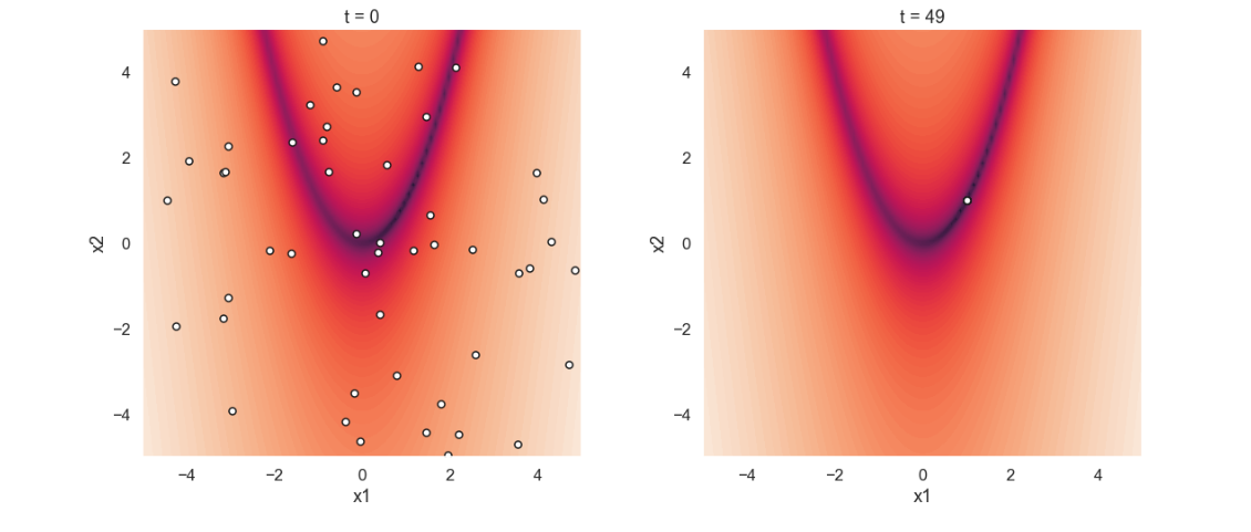
Time to look at the results! The plots below show the initial positions of each particle in the swarm as well as the positions after 50 loops.

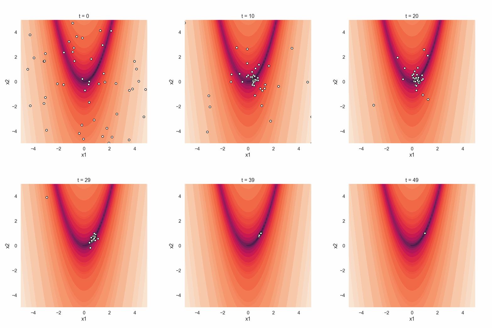
Starting off with the initial positions we see that the location of the particles are random. The picture from the last iteration shows that all particles are located at the global minimum of the function. This is realy nice since it looks like this sort of simple algorithm works quite well! Perhaps an even more interesting thing to show is the movement of the particle swarm during the iterations. Below is an animated gif showing just that.

Time to conclude
Rather short blog post this time. Anyhow I think that this particle swarm optimization algorithm is a really cool way to solve a minimization problem like the one we have looked at in this blog post. The idea behind the algorithm is quite easy and it was not much work at all to make an implementation from scratch in python. One of the reasons for the simplicity of the implementation is that the method does not need any calculation of the gradient for the function. This also means that there is no restriction on the function that it needs to be differentiable. Moreover, this optimization method is known to be fairly robust.
Well I guess that was all for this time and, as always, feel free to contact us at info@gemello.se