So, a new blog post! Alright!! Here we are going to make use of Bayesian statistics in order to make some $cash$. Well perhaps not but the blog post will take place at a (at least imaginary) casino. So, put on the tuxedo (or equivalent) and let's get ready.
S*ut up and take my money
So, we are at the casino and in front of you there are four different old fashioned slot machines known as one-armed bandits. You know, the ones with a handle on one side (the one-armed part) and it will most likely take all your money (the bandit part).

When you play one of the one-armed bandits there can be two different outcomes, either you “lose” i.e. you do not get any money back or you “win” i.e. you get some cash back from the machine. For simplicity a “win” will always be a fixed number of money and it is the same for all the four machines. What is different between the machines is the probability to “win” and these values are at the moment unknown to us.
So, here is the thing. You have a fixed number of times you can play and each time you play you have to choose one out of the four different machines that are in front of you. For sure, you would like to find the best machine i.e. the machine with the highest probability of a “win” and play that as much as possible but how do you do that? This is where Bayesian statistics will guide you on your path to the big bucks. (Just so you know, gambling is a really bad idea so don’t do that)
The python bandit
You know what, we just start right away with some coding! For this to work we need to define the probability of winning for each machine and we will use this to check our results when we are done.
Let's write a small function that simulates the playing of one out of the four machines! First some standard imports
import numpy as np
import matplotlib.pyplot as plt
import seaborn as sns

sns.set(context='talk')
Now, let's define a list that contains the probability of winning for each of the four machines
prob_win = [0.1,0.15,0.20,0.25]
These numbers are for sure made up since I believe the probability to win when playing a one armed bandit is much smaller. So the first machine, called machine 0 since we are using python :-), has a probability of 10% to produce a win and the last machine has a probability to win of 25%. Now the functions that simulates us playing one out of the four machines one time
def play_machine(prob_win,i):

    p = prob_win[i]

    if np.random.rand() < p:
        return 'W'
    else:
        return 'L'
Here i is a number between 0 and 3 that represents which machine that is played. The function will return either the letter 'W' that means you have won (alright!!) or the letter 'L' meaning you lost. Let's try it out by playing each machine 200 times and record the number of wins you got from each machine
nr_wins = np.zeros(len(prob_win))
for i in range(0,len(prob_win)):

    for _ in range(0,200):

        r = play_machine(prob_win,i)
        if r == 'W':
            nr_wins[i] = nr_wins[i] + 1
Ok, that was quite easy. Let's make a nice looking bar chart of the number of wins for each machine!
plot_colors = ['b','orange','g','r']

plt.figure(figsize=(8,5))
plt.bar([0,1,2,3],nr_wins,color=plot_colors,edgecolor='k')

plt.xticks([0,1,2,3])
plt.xlabel('Machine nr')
plt.title('# Wins')

plt.show()
and the plot
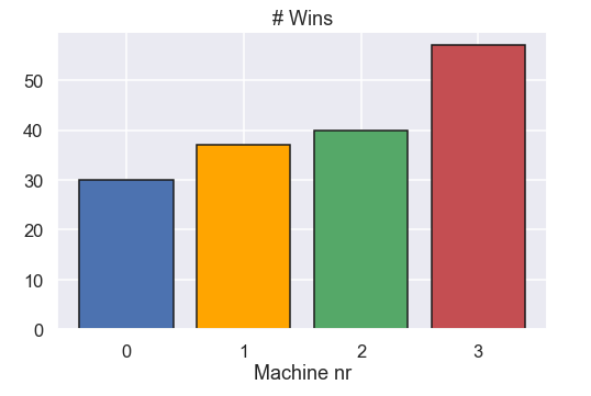
Ok! We see that we got the most wins from machine nr 3, nice! Counting the number of wins is for sure nice but wouldn't be much cooler if we had an estimate, including uncertainty, of the probability to win for each machine! This is where we step into Bayesian statistics.
Bayes rules!
We have actually done something similar in a previous post so feel free to check that out for a more in depth description. Anyhow, as we usually do we use Bayes rule to get an estimate of some quantity and Bayes rule looks like this
\[ p(H|D) = \frac{p(H) \cdot p(D|H) }{p(D)} \]
where \(H\) and \(D\) represent the hypothesis and the data, respectively. The thing to the left, \(p(H|D)\) is the posterior distribution and this is the thing that we are interested in. The stuff to the right of the equal sign is the prior, \(p(H)\), the likelihood function, \(p(D|H)\), and finally the normalizing constant, \(p(D)\).
So, basically what the equation above allows us to do is to update our belief about something when we see some data. In this specific case we start with some belief about the probability for a machine to produce a win and when we play a machine we get some data (a win or no win) and then update our beliefs about the machine. This is often called a Bayesian update.
So, what we need to do is to handle the three different terms to the right of the equal sign in Bayes rule above. Let’s start with the likelihood function \(p(D|H)\) since this perhaps is the hardest one. First of all, by the hypothesis, \(H\), we mean the probability to get a win from a machine. Now, the likelihood function will in this case answer the question: what is the probability to get a win/no win given that the probability of getting a win is \(H\)? So, as an example if the probability of getting a win, \(H\), is 30% what is the probability to get a win?? Well it must be 30%. And then, for the same \(H\) of 30% what is the probability to get a no win? Well it must be 1-0.3 = 70% This can be written in a small function:
def likelihood(H,D):

    if D == 'W':
        like = H
    else:
        like = 1 - H

    return like
Nice! Now, let’s look at the prior, \(p(H)\). Before we have played any of the machines we do not know anything about the probability for a machine to produce a win. So a reasonable prior for each machine is a complete flat one i.e. all probabilities of a win are the same.
Finally the thing on the bottom in the equation \(p(D)\). This can be seen as a normalizing constant so we can just calculate it so the posterior probability is summed up to 1 (100%).
Super, we have now defined all the components needed to use Bayes rule to make the Bayesian update. Let’s write a small function that actually does the Bayesian update.
def update_posterior(win_rate,Post,i,result):

    Posterior = np.copy(Post)
    post = Posterior[i]

    like = likelihood(win_rate,result)

    post = post*like           # update posterior
    post = post / np.sum(post) # normalize

    # store
    Posterior[i] = post

    return Posterior
The very first and last part is just making sure that we update the posterior distribution for the machine played (indicated by the variable i). The nice thing about a Bayesian update is that when you get additional data i.e. you play the same machine again you just use your current belief about the probability of getting a win as prior i.e. your posterior becomes the prior for the next Bayesian update.
So let’s do a similar thing as above to play each machine 200 times but instead of just counting the number of wins from each machine we do a Bayesian update about the probability for each machine to produce a win. To do this we just need to define four different posteriors and keep track of which machine that is played.
machine_played = np.zeros(len(prob_win))

win_rate = np.linspace(0,1,500)


# initiate
Posterior = []
for _ in range(0,len(prob_win)):
    Posterior.append(np.ones(len(win_rate))/np.sum(np.ones(len(win_rate))))

nr_wins = np.zeros(len(prob_win))


for i in range(0,len(prob_win)):

    for _ in range(0,200):

        # play machine
        r = play_machine(prob_win,i)

        # update posterior
        Posterior = update_posterior(win_rate,Posterior,i,r)

        # store number of wins
        if r == 'W':
            nr_wins[i] = nr_wins[i] + 1
And here is a plot of the different posterior distributions as well as the number of wins for each machine.
plt.figure(figsize=(18,6))

plt.subplot(1,2,1)
for j in range(0,4):
    plt.plot(win_rate,Posterior[j],label='Machine '+ str(j),c=plot_colors[j],lw=3)
plt.legend()
plt.xlabel('Probability to win [-]')
plt.title('Posterior distribution')

plt.subplot(1,2,2)

plt.bar([0,1,2,3],nr_wins,color=plot_colors,edgecolor='k')
plt.xticks([0,1,2,3])
plt.title('# of wins')
plt.xlabel('Machine nr')

plt.show()
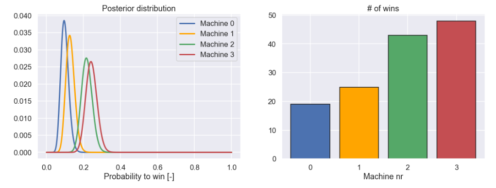
So, what we can learn from the posterior distributions for the four different machines is that we probably should not play machine 0 and 1 anymore because it seems very unlikely that these are the best machines to be played.
Now we have come to the perhaps most interesting part of the blog post where we will try to give an answer to the question posted in the beginning of this post. What strategy should we have to, in the fastest way, find the best machine to play?
Ladies and gentlemen place your bets
Now, here is the deal. You have a fixed number of times you can play any of the four machines you have in front of you, let’s make this number 1000 times. For sure we would like to play the best machine as many times as possible but how can this be done? In the example above we used 800 out of the 1000 times and we found that machine number 0 and 1 are probably not the best one
As I see it, the sort of bad thing with the strategy that was used above is that we set a fixed number of times that we play each machine so the uncertainty of the estimations are similar for all machines. This is represented by the similar width of the four different posteriors. A perhaps better idea is to play a machine, update the posterior and then, based on the things we know, decide which machine to play next. By using this approach we can probably avoid “wasting” time playing the bad machines, since as soon as we are pretty sure it is not the best one we do not need to play it anymore.
So, how exactly are we going to do this? Well, here is one idea. When we decide on which machine to play next we draw a sample from each of the machines' posteriors. Then we play the machine with the highest sample value. Sounds simple right! Let’s just write a small function that will do just that
def choos_machine(win_rate,Posterior):

    post_check_prob_win = np.zeros(len(Posterior))
    for j in range(0,len(Posterior)):

        Post = Posterior[j]
        post_check_prob_win[j] = np.random.choice(win_rate,p=Post)

    return np.argmax(post_check_prob_win)
There are some really nice features with a strategy like this one! In the beginning when we do not know so much about any of the machines i.e. the posterior are pretty wide for all machines, we tend to play each machine by the same probability. This means that we have more of an exploring strategy. However, when we know more about the different machines we tend to play the ones that are better with a higher probability i.e. we are having more of an exploiting strategy. Nice! Let’s put it all together in code.
# initiate
nr_machine_played = np.zeros(len(prob_win))
win_rate = np.linspace(0,1,500)

# Prior distribution
Posterior = []
for _ in range(0,len(prob_win)):
    Posterior.append(np.ones(len(win_rate))/np.sum(np.ones(len(win_rate))))

# For plotting
machine_played_plot = []
machine_played_plot.append([0,0,0,0])
polsterior_plot = []
polsterior_plot.append(Posterior)


# Play
nr_play = 1000

for n in range(0,nr_play):

    i = choos_machine(win_rate,Posterior)
    result = play_machine(prob_win,i)
    Posterior = update_posterior(win_rate,Posterior,i,result)

    nr_machine_played[i] = nr_machine_played[i] + 1

    machine_played_plot.append(np.copy(nr_machine_played))
    polsterior_plot.append(Posterior)
Alright, not that much code. Believe it or not but we are actually done, so let’s plot the final result.
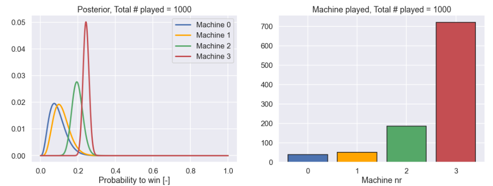
This is really nice. Out of the 1000 times we could play a machine we played nr 3, i.e. the best one, more than 700 times.
Just as a final illustration let’s show an animation of how the different machines were played during the 1000 attempts as well as how the posterior distributions evolved.
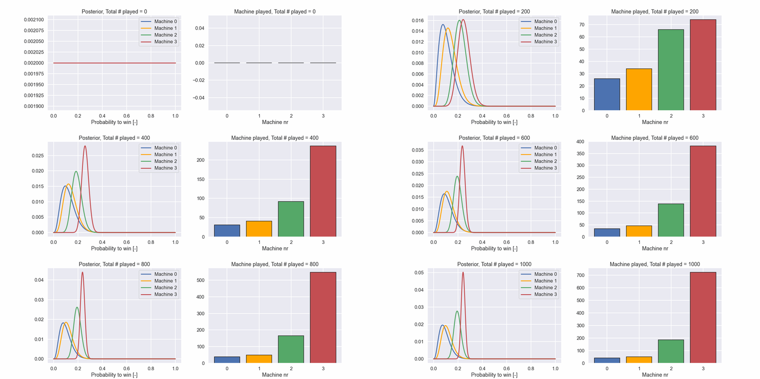
Here we can clearly see that in the beginning all machines are played rather evenly but at a certain point the machines with a lower probability to produce a win are played more and more seldom. Exactly according to the plan!
Time to conclude
Even though many blog posts have been about statistics this is the first one that took place at a casino. For sure you can imagine a situation outside a casino where something like this can be useful as well. What I really like about this is the sort of adaptive sampling strategy where you do not need to give a detailed test plan at the start of the experiment. You always take your current knowledge into consideration when deciding the next step.
Well I guess that was all for this time and, as always, feel free to contact us at info@gemello.se