New blog post, exciting! In this post we will have a closer look at a gaussian process with the aim of simulation thickness variation in a sheet of material.
So what is Bayesian optimization?
Perhaps a good place to start is to give a general description of Bayesian optimization. Well, since it is optimization we are dealing with, the aim is to find some sort of optimal point for some function. It will be assumed that this function is a "black box" function i.e. we do not have any information about the function (or its gradients). The only thing we can do is give it some values of the input variables and the black box function will return a value associated with the input values.
One of the situations where Bayesian optimization can be a good candidate is when the evaluation of the black box function is really expensive to evaluate. For instance, drilling for oil is really expensive and you can not afford to do that many function evaluations. Another example could be that the black box function is a lab experiment that takes like 6 months to evaluate (like optimizing the properties of a certain crop) so time is the limiting factor. We will late on use Bayesian optimization to optimize some response from a finite element model which also has a tendency to be time and resource intensive (but still cheaper than building the real structure and evaluate it)
So, the steps that is included in the Bayesian optimization algorithm are:
- Start with a small number of randomly selected points
- Use these points to evaluate a surrogate function
- Start an iteration loop
- Select a new additional point by use of an acquisition function
- Re-evaluate the surrogate function
- Continue until some termination criteria is met
That’s it!
We will spend the following next two subsections on the surrogate function and the acquisition function respectively but before we do that let’s just say a word or two about the termination criteria.
As mentioned before, this optimization algorithm is favorable in the case where the black box function is expensive to evaluate so one sort of practical approach to a termination criteria is to, in advance, decide on a budget i.e. the number of function evaluations that I can afford. Of course, one can terminate the iteration before reaching the budget if for instance the algorithm is always choosing the same point to evaluate in the next iteration.
So let’s start with the surrogate function!
Gaussian process - (un)conditional love
A gaussian process is to be considered the "standard" surrogate function when doing bayesian optimization. We have actually already looked at Gaussian processes In this previous blog post so perhaps reading through that post could be a good idea. Anyhow, let’s just look at some basics when it comes to Gaussian processes again.
From the blog post above we used a definition similar to this:
In probability theory and statistics, a Gaussian process is a stochastic process (a collection of random variables indexed by time or space), such that every finite collection of those random variables has a multivariate normal distribution, i.e. every finite linear combination of them is normally distributed.
Or, in a mathy way of expressing it
\[ X \sim \mathcal{N}(\mu,\,\Sigma) \]
The quantity \(\mu\) tells something about the average values and \( \Sigma \) known as the covariance matrix. More on this later.
The next “trick” was the visualization of the high dimensional data where we simply put the variables along an axis and marked the value on the other axis, like this
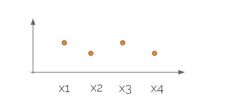
Note that this is just one sample from a multivariate normal distribution and if we took a new sample it would look different. If we took many samples the values for each variable would be described by a normal distribution with corresponding mean and standard deviation.
Finally, and perhaps most importantly, the correlation between the different variables was a function of the distance between them i.e. high correlation if the points are close and low correlation if the points are far away from each other.
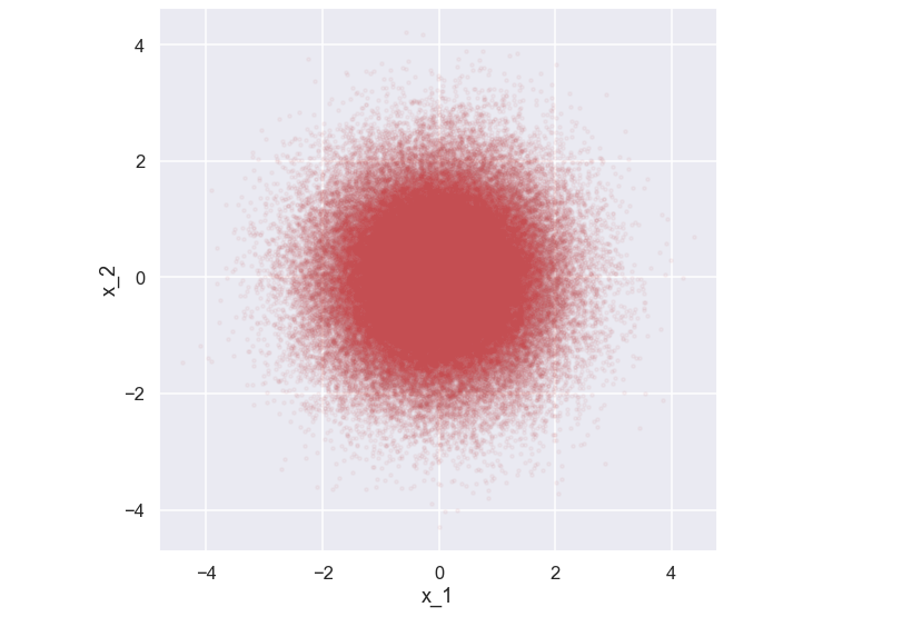
Now, here comes some new stuff. In order to use a Gaussian process as the foundation of our surrogate model we need to (at least loosely) understand what is happening when we have some data involved i.e. when we know the value of the black box function in some locations. We will not go into details on this but it is still a good idea just to have some intuition about what is happening. So, let’s look at the simplest example possible - an example with two variables. As discussed above let’s generate some data from a 2D Gaussian distribution where both \( x_1\) and \(x_2\) have zero mean and 1 as standard deviation. Moreover, no correlation between the variables is present. Let's start coding by doing some standard imports
import os
import shutil
import numpy as np
import scipy as sp
import matplotlib.pyplot as plt
import seaborn as sns

sns.set(context='talk')
Some code
# Data for multivariate data
mu1, mu2 = 0.0, 0.0
S11, S22, S12 = 1.0, 1.0, 0.0
p = np.random.multivariate_normal([mu1,mu2],[[S11,S12],[S12,S22]],100000)

plt.figure(figsize=(9,9))
plt.scatter(p[:,0],p[:,1],color='r',s=10,alpha=0.05)
plt.xlabel('x_1')
plt.ylabel('x_2')
plt.axis('equal')
plt.show()
And then the plot
Now, what would happen if we knew the value of e.g. \(x_1\) i.e what would the probability distribution for \(x_2\) look like given a value of \(x_1\)? Just for the discussion, let’s assume that \(x_1 = 1\). So, the simple and approximative solution to this would just be to look at the picture above and then just keep the data points where x_1 = 1 (given some small variation). Let’s try that out.
mu1, mu2 = 0.0, 0.0
S11, S22, S12 = 1.0, 1.0, 0.0
p = np.random.multivariate_normal([mu1,mu2],[[S11,S12],[S12,S22]],100000)

# condition on x_1
x1_cond = 1
dist_x1_cond = p[np.isclose(p[:,0],x1_cond,atol=0.05),1]


plt.figure(figsize=(20,9))

plt.subplot(1,2,1)
plt.scatter(p[:,0],p[:,1],color='r',s=10,alpha=0.1)
plt.vlines(1,-3.5,3.5,'k',lw=5)
plt.xlabel('x_1')
plt.ylabel('x_2')
plt.xlim(-4,4)
plt.ylim(-4,4)

plt.subplot(1,2,2)
plt.hist(dist_x1_cond,bins=np.linspace(-4,4,40),orientation="horizontal",color='r',edgecolor='k')
plt.ylabel('x_2')

plt.show()
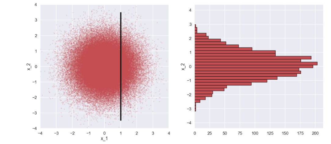
Ok, what have we here? In the picture to the right we see a histogram of \(x_2\) which kind of looks like a normal distribution. One can imagine that the mean and standard deviation for this distribution, \(p(x_2|x_1=1)\), will be a function of the mean and standard deviation of \(x_2\) as well as the conditional value of \(x_1\). Now, we try something different. What if there is a correlation between \(x_1\) and \(x_2\)? Let’s try that out with some minimal changes to the code
mu1, mu2 = 0.0, 0.0
S11, S22, S12 = 1.0, 1.0, 0.9
p = np.random.multivariate_normal([mu1,mu2],[[S11,S12],[S12,S22]],100000)

x1_cond = 1
dist_x1_cond = p[np.isclose(p[:,0],x1_cond,atol=0.05),1]

plt.figure(figsize=(20,9))

plt.subplot(1,2,1)
plt.scatter(p[:,0],p[:,1],color='r',s=10,alpha=0.1)
plt.vlines(1,-3.5,3.5,'k',lw=5)
plt.xlabel('x_1')
plt.ylabel('x_2')
plt.xlim(-4,4)
plt.ylim(-4,4)

plt.subplot(1,2,2)
plt.hist(dist_x1_cond,bins=np.linspace(-4,4,40),orientation="horizontal",color='r',edgecolor='k')
plt.ylabel('x_2')

plt.show()
Here is the plot
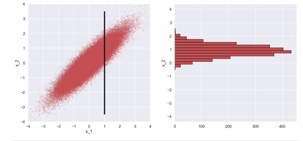
Interesting! If we look at the histogram of \(x_2\) when \(x_1\) and \(x_2\) are (highly) correlated the standard deviation of \(p(x_2|x_1=1)\) is much smaller than for the case where they are not correlated. Moreover, the mean value of \(x_2\) is is shifted close to the value of \(x_1\) for the case of high correlation whereas for the case with no correlation, the mean of \(p(x_2|x_1=1)\) is still close to \(0\).
So, what does this mean?
Well, remember from above that the idea with the gaussian process is that points that are close to each other have high correlation whereas points that are located far away from each other have low correlation. So, if we know the value of the black box function for a certain location we can be more certain about the value of the black box function at locations that are close by. That is, we assume that the mean value of a nearby point is close to the known value of the black box function. Moreover, the standard deviation of the nearby point is quite small compared to a point that is situated far away from the known location.
There are actually closed form expressions for the mean and standard deviation for arbitrary points when conditioning for some data, have a look here for instance. However, we are going to use scikit learn to do all the heavy lifting when it comes to the gaussian process. More on this in the examples that will follow.
Aquisition function - where to go next?
Now when we have the surrogate model let’s continue with the acquisition function. As mentioned above, the idea of the acquisition function is to find the next point to evaluate. Since we are using a gaussian process as the surrogate model, we have estimates of both the mean and the standard deviation at any arbitrary point which is pretty cool. There are several versions of the acquisition function but the one we are going to use in this blog post looks like this (for the case where we would like to maximize the black box function)
\[ a = \mu + \alpha \sigma \]
where \(\alpha\) is a scale factor. This acquisition function is called Upper Confidence Limit or UCL.
When we are looking for the next point to evaluate there are basically two things that we can do. The first thing is to look in the area near known points where the black box function has high values (in the case that we would like to maximize the value of the black box function). This can be referred to as exploitation and is represented by the first part i.e. the mean value in the acquisition function. Secondly, we can look in the area where we don’t know that much about the black box function with the hope that there might be something interesting. This is referred to as exploration and is represented by the standard deviation part in the above acquisition function. The parameter \(\alpha\) is a parameter that controls the mix between exploration and exploitation
So, basically the most interesting point i.e. that one we would like to evaluate in the text step is the point which maximizes the acquisition function.
OK! Now we have a better understanding of what should be going on, let's have a look at two examples. The first example is a sort of toy example where we actually know the black box function, this is just to get a feel for how the optimization algorithm is working. In the second example we are moving a bit closer to reality (but still a sort of simple example) where the black box function includes a finite element model of a simplified crash box.
Oh, show me (Heaven) an Example
So, let’s try to put together the different steps involved in Bayesian optimization. In this first example we are going to use a rather simple 1-D function as the black box function. To be fair, it is not really a “black box” function since we will define it explicitly but the idea is to show how the algorithm works.
The function that will act as the black box function is defined as:
\[ f(x) = x \sin(x) \]
so, something that is oscillating with increasing amplitude. Let’s code this as a separate function
def my_func(X):
    y = np.squeeze(X * np.sin(X))
    return y
Now, let's plot the function.
X = np.linspace(0,10,500).reshape(-1,1)
f_X = my_func(X)

plt.figure(figsize=(15,5))
plt.plot(X, f_X, label=r"$f(x) = x \sin(x)$", linestyle="dotted",lw=3)
plt.legend()
plt.xlabel("$x$")
plt.ylabel("$f(x)$")
plt.ylim(-12,12)
plt.title("Function to maximaize")
plt.show()
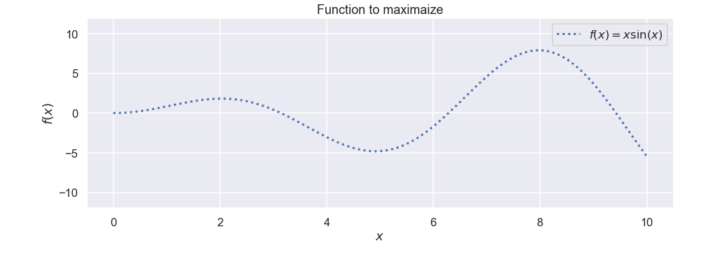
Nice. We can see that the function has its maximum value somewhere close to \(x=8\).
Now we have come to the surrogate function and as mentioned above we will use scikit learn to model the Gaussian process. First some imports
from sklearn.gaussian_process import GaussianProcessRegressor
from sklearn.gaussian_process.kernels import RBF
Then we define the property of the kernel i.e. the correlation between the different variables which control the smoothness of the function. We also make an instance of the model.
kernel = 5 * RBF(length_scale=1.0, length_scale_bounds='fixed')
gaussian_process = GaussianProcessRegressor(kernel=kernel, n_restarts_optimizer=0)
Now, to check if the definition of the kernel is sort of OK we can take samples from the gaussian process before we have seen any data. Let’s do that and plot the results
sample_prior = gaussian_process.sample_y(X,4)


# Plotting the samples

plt.figure(figsize=(12,6))
for i in range(0,4):
    plt.plot(X,sample_prior[:,i],lw=3,label='Sample from Prior '+ str(i))
plt.xlabel("$x$")
plt.ylabel("$f(x)$")
plt.ylim(-8,8)
plt.legend()
plt.show()
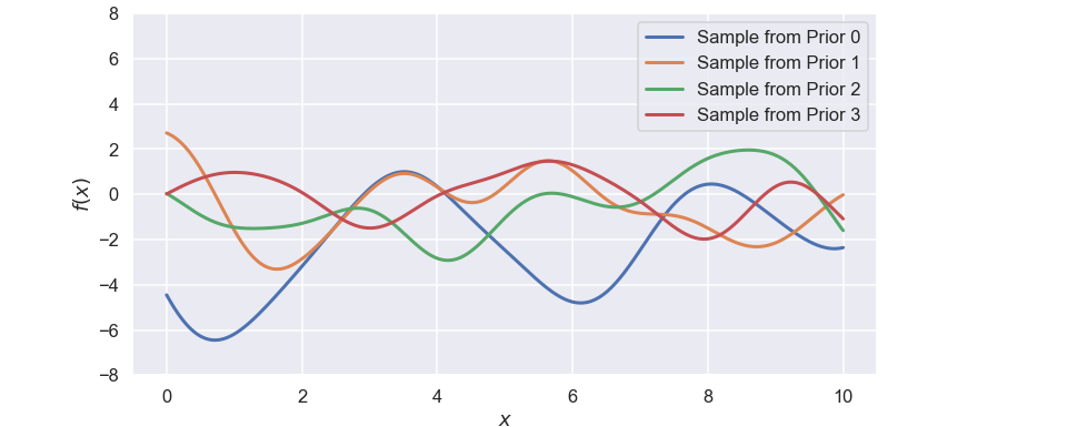
Well, this seems quite reasonable to me, each sample looks a bit different but the amount of “wiggelness” is ok to me, i.e. they are not too wiggly but they do change over the studied interval.
We have now reached the part where we show the Gaussian process some data and as stated above it is a good starting point to take a few random points where the black-box function is evaluated. In this case let’s start with \(x=[1,5]\). The conditioning on the data part is done by utilizing the gaussian_process.fit() method and it is all done with a few lines of code below.
X_train =[1,5]
Y_train = my_func(X_train)

gaussian_process.fit(np.array(X_train).reshape(-1,1), Y_train)
So, let’s do some prediction. This is done by the gaussian_process.predict() method where we input the points where we would like to have predictions. In this case it is a lot of of points that are evenly spread out over the studied interval. It would look something like this
mean_prediction, std_prediction = gaussian_process.predict(X, return_std=True)
The output from this is that for each point in the X vector we get a mean value and a standard deviation. Let’s write some lines of code that plot this in a nice way.
X_scatter = []
Y_scatter = []
pdf_scatter = []

y = np.linspace(-10,10,200)

for i in range(0,len(X)):

    pdf = sp.stats.norm.pdf(y,mean_prediction[i],std_prediction[i])

    Y_scatter.append(y)
    X_scatter.append(y*0 + X[i])
    pdf_scatter.append(pdf)


plt.figure(figsize=(15,8))
plt.scatter(X_scatter,Y_scatter,c=pdf_scatter,vmin=0,vmax=0.2,cmap='viridis')
plt.plot(X,mean_prediction,'w-',lw=4)
plt.plot(X,mean_prediction+std_prediction*2,'w-',lw=1)
plt.plot(X,mean_prediction-std_prediction*2,'w-',lw=1)

plt.show()
and the plot
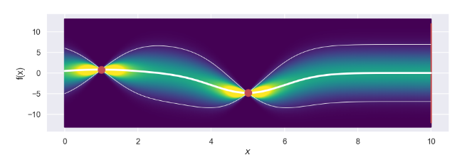
Sweet, the thicker white line represents the mean for each point and the two thinner white lines visualize an interval of +/- two standard deviations from the mean value. What we can clearly see, which is expected, is that for the two data points we have so far the uncertainty i.e. the standard deviation is zero. To the contrary, points that are far away from the current data points have a larger uncertainty (which also is expected).
Nice! Let’s take the next step of calculating the acquisition function. Since we now have both the mean value and the standard deviation at each point we can simply calculating the acquisition function according to the definition above
alpha = 3.00
acquisition_function = mean_prediction + alpha*std_prediction
Let’s plot it as well!
plt.plot(X,acquisition_function,'b',lw=5)

plt.plot(new_x,np.max(acquisition_function),'ro',ms=15)

plt.ylabel('Acquisition function')
plt.xlabel("$x$")
plt.show()
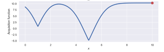
Where we have used an \(\alpha = 3\) which of course is a bit arbitrary, but I think/hope that this will give a nice mix between exploration and exploitation as discussed above. Now for the fun part, which is the point that we should evaluate in the next step? Well, for this we “just” need to find the max of the acquisition function. In this case this is quite easy, we can use the numpy.argmax() function. So the next point will be
new_x = X[np.argmax(acquisition_function)][0]
This is the point that is highlighted by the red dot in the figure above.
Sweet! Believe it or not but we have now defined all the components needed to use Bayesian optimization in order to find the maximum of our black-box function (which in this case is not a real black box since we know the function…). So let’s put all the code snippets together, run it for a few iterations and see what is happening. First the code:
gaussian_process = GaussianProcessRegressor(kernel=kernel, n_restarts_optimizer=0)
gaussian_process.fit(np.array(X_train).reshape(-1,1), Y_train)

mean_prediction, std_prediction = gaussian_process.predict(X, return_std=True)

alpha = 3.00
acquisition_function = mean_prediction + alpha*std_prediction
new_x = X[np.argmax(acquisition_function)][0]

X_scatter = []
Y_scatter = []
pdf_scatter = []

y = np.linspace(-13,13,200)
pdf = sp.stats.norm.pdf(y,mean_prediction[0],std_prediction[0])

for i in range(0,len(X)):

    pdf = sp.stats.norm.pdf(y,mean_prediction[i],std_prediction[i])

    Y_scatter.append(y)
    X_scatter.append(y*0 + X[i])
    pdf_scatter.append(np.nan_to_num(pdf))


plt.figure(figsize=(15,10))
plt.subplot(2,1,1)

plt.scatter(X_scatter,Y_scatter,c=pdf_scatter,s=2,vmin=0,vmax=0.2,cmap='viridis')

plt.plot(X,mean_prediction,'w-',lw=4)
plt.plot(X,mean_prediction+std_prediction*2,'w-',lw=1)
plt.plot(X,mean_prediction-std_prediction*2,'w-',lw=1)

plt.plot(X_train,Y_train,'ro',ms=15)

plt.vlines(new_x,-12,12,color='r',lw=3)

plt.xlabel("$x$")
plt.ylabel('f(x)')

plt.subplot(2,1,2)
plt.plot(X,acquisition_function,'b',lw=5)
plt.plot(new_x,np.max(acquisition_function),'ro',ms=15)

plt.ylabel('Acquisition function')
plt.xlabel("$x$")

plt.savefig('Test_1D_'+str(iter_nr))

plt.cla()
iter_nr = iter_nr + 1

X_train.append(new_x)
Y_train = my_func(X_train)
And then an animated gif with the different steps.
Awesome! What we can see is that in the beginning when there is a large uncertainty in several areas the algorithm will do more exploring but as the uncertainty decreases it will be more focused around the area where we have found the max value.
Well, this was encouraging, let’s have a look at a more realistic example.
Crash! Boom! Bang!
In the example above the black-box function was not really a black-box function. This was just in order for us to be able to judge the performance of the algorithm. So, let's look at something different, in this case a finite element model of a simplified crash box.
This model setup is taken from this web page with some small modifications.
The tube is impacted by a rigid plane(from left in the picture above) with some mass at a certain speed and the purpose of the crash box is to absorb the impact energy in a smooth way. Moreover, the tube is attached to a rigid wall on the right hand side of the picture. An animated gif of an impact sequence is shown below.
So, if we would look for the “smoothest” way possible to absorb the energy what would that mean? Well, if the crash box was really rigid there would be a really high force just after the mass hit the crash box. To the contrary, if the crash box was really thin and made out of paper it would not reduce the speed of the mass at all, that would happen when the mass hit the rigid wall to the right. One interesting thing to look at would be the maximum acceleration of the mass during the whole impact sequence and then do some modification to the crash box in order to minimize this quantity.
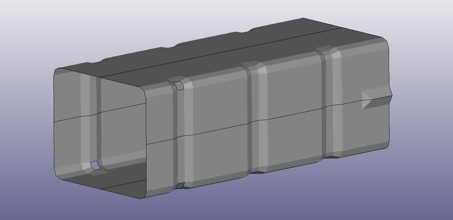
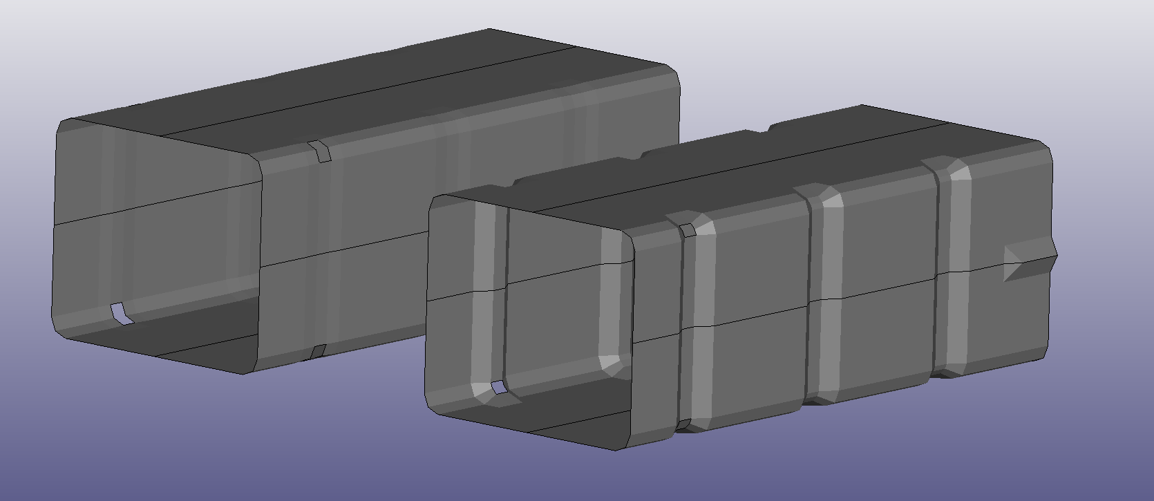
We will not make it too complicated here when it comes to what properties of the crash box to change, let’s look at the impact from thickness and shape. By thickness we just mean the thickness of the metal that forms the crash box. The shape is perhaps a bit more complicated but by shape we mean the depth of the predefined areas where the crash box will fold. We will use a scale factor called \(\overline{shape}\) (that varies between 0 and 1) to control the shape and below are two pictures with \(\overline{shape} = 0\) (left) and \(\overline{shape} = 1 \) (right).
The thickness of the crash box is defined in the *SECTION_SHELL card. Here we have also introduced a scaled parameter, \( \overline{thickness} \), which varies between 0 and 1 and this corresponds to a real thickness that varies between 0.5mm and 2.5mm
To generate a finite element model with the specific shape factor and thickness factor we simply write an additional file with this information and then use the *INCLUDE card in the main file. Below is the code that writes the included file.
def write_input(run_nr,scale_bar,thickness_bar):

    # Make new directory and copy files
    wai = os.getcwd()
    na = 'Bayes_opt_' + str(run_nr)

    source_dir = wai+os.sep+'FEM_Files'
    destination_dir = wai+os.sep + na
    shutil.copytree(source_dir, destination_dir)


    # morphing
    sorted_nodes = np.loadtxt('Sorted_node_coords.k',comments='*',delimiter=',')
    nodes_flat     = np.loadtxt('Sorted_node_coords_flat.k',comments='*',delimiter=',')
    diff = sorted_nodes - nodes_flat
    scale = 0.1 + scale_bar * 1.1
    new_nodes = nodes_flat + scale*diff

    # thickness
    t = 0.5 + thickness_bar*2.0

    # write input

    f = open(wai+os.sep+na+os.sep+'Nodes_coords_and_t.k','w')

    f.write('*KEYWORD\n')
    f.write('*NODE\n')


    for i in range(0,len(new_nodes)):
        f.write(str(int(new_nodes[i,0])) + ', ' +
                str(np.round(new_nodes[i,1],5)) + ', ' +
                str(np.round(new_nodes[i,2],5)) + ', ' +
                str(np.round(new_nodes[i,3],5)) + '\n')


    f.write('*SECTION_SHELL\n')
    f.write('1,2,,3.000\n')
    f.write('%5.4f, %5.4f, %5.4f, %5.4f\n' % (t,t,t,t))
    f.write('*END')
    f.close()
And the additional include command in the main file
*INCLUDE
Nodes_coords_and_t.k
Elements.k
Here, Elements.k is just a file that keeps the information about the element connectivity.
Finally, we need to calculate the thing we like to minimize. The acceleration of the mass is written to the text formatted nodout file so we can read it quite easily by a helper function defined below.
def read_nodout(run_nr):

    wai = os.getcwd()
    na = wai+os.sep+'Bayes_opt_' + str(run_nr)
    f = open(na + '\\nodout')

    time_array = []
    z_acceleration_array = []


    read_time = 11
    read_value = 14

    for i in range(0,68000):
        lines = f.readline()
        if i == read_time:

            time_array.append(float(lines[-17:-2]))

            read_time = read_time + 14

        if i == read_value:

            z_acceleration_array.append(float(lines[107:107+11]) )
            read_value = read_value + 14

    f.close()

    return np.array(time_array), np.array(z_acceleration_array)
What we have now is the acceleration as a function of time and from this we can simply find the maximum value using numpy.max().
So, I think we are done with the setup of the model, let’s do some Bayesian optimization! Similar to the test example above we have to initiate the gaussian process including the kernel function. When this is done it could be a good idea just to take some samples from the gaussian process just to make sure that it looks ok.
X = []

for x1 in np.linspace(0.0,1.0,50):
    for x2 in np.linspace(0.0,1.0,50):
        X.append([x1,x2])

X = np.array(X)

kernel_n = 1 * RBF(length_scale=0.3, length_scale_bounds='fixed')
gaussian_process_2D = GaussianProcessRegressor(kernel=kernel_n, n_restarts_optimizer=10,normalize_y=True)

sample_prior = gaussian_process_2D.sample_y(X,3)
Let’s plot the samples, since we have two parameters in this example we can visualize the result in a scatter plot
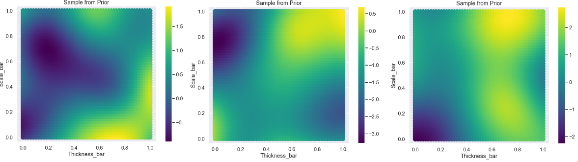
Ok, nice! This seems to be reasonable, some variation going on but not too much.
Next we have the acquisition function. We are going to use the same form as in the previous example but since in this case we would like to minimize the acceleration we will look at the lower confidence limit. This is done by just switching the + sign to a - sign in the acquisition function. Why not have a look at the acquisition function after we have taken 6 randomly selected data points at the start of the optimization process.
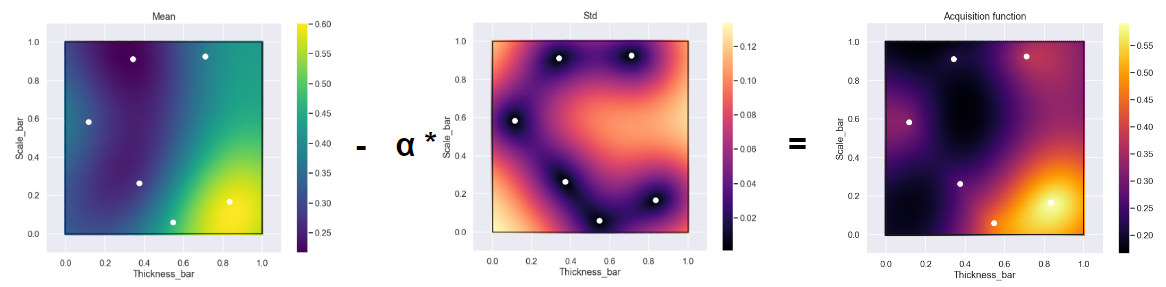
Here we have plotted the mean and the standard deviation just to visualize the two separate contributors of the acquisition function. What is expected is the standard deviation to be really small at the location of the data points which is highlighted by the middle image. So, to find the next point to evaluate we simply find the location of the minimum for the acquisition function (similar to what we did in the first example but there we looked for the maximum).
I think we have everything we need now to start running the Bayesian optimization loop! The code for one optimization iteration is found below.
kernel = 1 * RBF(length_scale=0.3, length_scale_bounds='fixed')
gaussian_process_2D = GaussianProcessRegressor(kernel=kernel, n_restarts_optimizer=10,normalize_y=True)

gaussian_process_2D.fit(np.array(X_points_2D),np.array(Y_points_2D))

mean_prediction_2D, std_prediction_2D = gaussian_process_2D.predict(X, return_std=True)


acquisition_function_2D = mean_prediction_2D - 1*std_prediction_2D

idx_min = np.argmin(acquisition_function_2D)


write_input(i,X[idx_min,0],X[idx_min,1])


# ------- Run main Ls-Dyna file


X_points_2D.append([X[idx_min,0],X[idx_min,1]])

time,z_acc = read_nodout(i)
z_acc_list.append(z_acc)

Y_points_2D = np.max(np.array(z_acc_list),axis=1)

i = i + 1
Where the counter, \(i\), was initiated at value \(i=0\) before the first iteration step.Note that the code should be run in different sections: The first part ends after the write_input() command. The second part is to run the Ls-Dyna main file for the current parameters. Then, finally, the results file is loaded and the maximum acceleration is calculated.
Let’s have a look at an animated gif for the optimization process.

So, what is going on here?
For sure points have been spread out over the whole domain (the exploration part) but the density of points seems to be higher in a region where \( \overline{thickness} \) is somewhere between \(0.15\) and \(0.35\). This is also the area where the points with the lowest maximum acceleration are found (exploitation part).
Just to get some more understanding of what is going on let’s have a look at three different data points, two bad ones and one good. In the figure below the three points are given as well as their acceleration curve as a function of time.
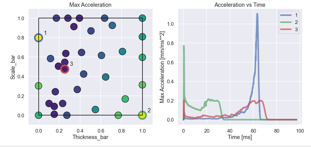
What we can see is that point nr 1 has really low acceleration in the first half or so of the impact (i.e. almost no loss of speed) and then the acceleration goes crazy high as the mass approaches the rigid wall at the end of the crash box. Definitely not an optimal design. For point 2 it is the other way around. Here there is really high acceleration at the beginning of the impact and after this it drops quite quickly down to zero (the mass is at rest). This is also not optimal since we have probably not used the crash box full potential. Finally, the third point looks really nice where there is some higher acceleration in the beginning and in the and the two peaks are approximately of the same magnitude. To even further understand what is going on let’s look at a picture of the three different configurations as well as an animated gif of the impact process.
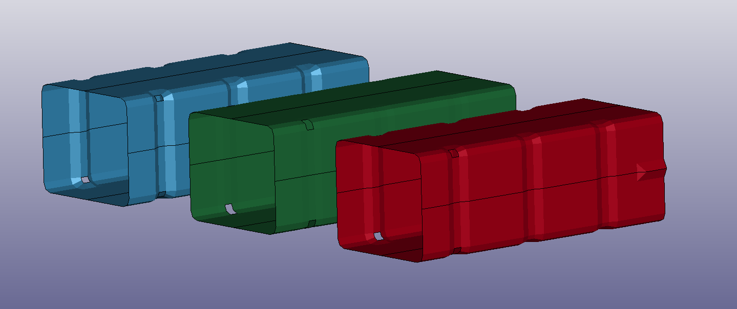
It is quite obvious that the crash box to the left is not doing a good job since basically all retardation of the mass is done when the mass more or less hits the rigid wall where the crash box is attached. For the green crash box it is clear that we have not used the full potential since we only use a fraction of the tube distance to stop the mass. Whereas the red crash box to the right in the picture seems to be absorbing the crash energy evenly during the complete impact process.
Time to conclude
A long blog post this time. Hope that the idea of Bayesian optimization is a bit more clear now. I think this method is quite cool since it offers this mix between exploration and exploitation. I also like that it is sort of dynamic when deciding where to go in the next step. In a standard design of experiment setup you would decide on all points to evaluate in advance and not take advantage of the results during evaluation. Finally, I also think it was cool to use a simple finite element model as an example since the finite element method is what I use more or less every day in my work.
Well, that was all for this time! I you would like to get in contact please drop an email at info@gemello.se.