Time for a new blogpost and the first post on the subject of artificial intelligence (AI).
What is learning?
We will here look into a specific case of machine learning. As you may know, there basically exist three types of machine learning algorithms:
- Supervised Learning
- Unsupervised Learning
- Reinforcement Learning
So what is the fundamental difference when it comes to reinforcement learning? In both supervised and unsupervised learning, we start from some kind of data from a dataset in order to create a model. Then hopefully the model will still work satisfying when exposed to data that were not part of the training data.
For reinforcement learning, there simply does not exist any data to begin with. What is available is some kind of environment that can be interactive with. After this interaction, some kind of feedback will be given. From this trial and error situation, we will now try to figure out how this environment works. The goal is to maximize some kind of long term reward. An illustration can be seen below.
Here we have the Agent, the one doing the interaction with the environment. The word “agent” is a rather good word since it has authority to do some actions depending on the current situation, described by the State. The environment will then send two things back: Some feedback, Reward, and a new state given as a consequence of the action previously taken. It is worth noting that the reward is not necessarily a positive one. If the agent would be standing at the edge of a cliff and decide to jump, most likely the reward will be negative.
How to figure things out??
OK, so we now have an agent interacting with the environment and the agent get some feedback from interacting with the environment. But how do we get from here to actually “learning” stuff? Well, first we need to figure out what we want to accomplish. As in life in general, this can be a simple or impossible question to answer. To make things easier, why not look at a simple example of the environment?
In this example, we are at the casino where we going to interact with one armed bandits. And to make things a bit more interesting, let’s say that we interact with 10 different ones.
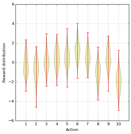
If you right now have some déjà vu, you are right. We have looked at a similar problem previously but limited to only four machines. Also, the rewards that gets out of the bandits is a bit different. While in the previous blog post the output was either win or no-win, in the case the output is an amount of “cache”. Our mission is here to find the machine with the highest output and then play that machine as often as possible. To make this problem even more interesting, the reward from the different machines has some randomness to them, so if we play the same machine on multiple occasions, the rewards will not be the same. Below you can se the output from interacting 200 times with each of the machines.

The output from the different machines is clearly overlapping, but bandit number 6 look to be the best choice. And just to be clear: Action 6 refers to playing machine number six. As a first step, let’s write some code representing the 10 bandits. To do so. Let’s create a class for the bandits:
class Bandit10:
    def __init__(self, epsilon=0.):

        # Initiate some stuff
        self.indices = np.arange(10)
        self.epsilon = epsilon
        self.time = 0
        self.average_reward = 0

    def reset(self):
        # real reward for each action
        self.q_true = np.random.randn(10)

        # startingvalue for estimated reward
        self.q_estimation = np.zeros(10)

        # reset time
        self.time = 0

        # counter for times for each action
        self.action_count = np.zeros(10)

        # what action is the best?
        self.best_action = np.argmax(self.q_true)
So what is going on here? First of all, there is one parameter, epsilon that we at the moment have no clue what those are. Let’s hope this gets clarified as this post goes on. Then there is a method called reset. What this method do is just to create a set of 10 bandits and initiate some variables. q_true is the true average for the different bandits and q_estimations is our estimation of the same property. In the beginning we do not know anything about the different machines so let’s just initiate q_estimations to zeros. Then we would like to keep track on the number of times we have played the different machines and also know which bandit is acutely the best one. Ones the setup is done, let’s continue to discuss some details on the learning process to find the best bandit.
As mentioned earlier, our mission is to find the best bandit and then play that one as much as possible in order to maximize our reward, but how to do this more in detail? Well, one way to do this is simply to look at our estimation of the mean (q_estimation) and just play the machine that has the highest estimated mean. This kind of strategy even has a name and is called the greedy action. When we select any of these actions we say that you are exploiting your current knowledge of the value of the actions. If we instead selected some on the nongreedy actions, then you are exploring, because this enables us to improve our knowledge of the system (the bandits). Exploitation is the right thing to do to maximize the reward in the short run, but exploration may produce a greater total reward in the long run. It seams reasonable that there exist some kind of optimal mix of the two, but how can we find this mix?
In the mix
To investigate this, we first need to take a look at how we estimate value for the different actions. One intuitive way of doing this is simply to look at the sample average, i.e.
$$ Q_t(a) = \frac{\sum_{i=1}^{T}R_i \cdot \mathbb{1}_{A_i=a}}{\sum_{i=1}^{T}\mathbb{1}_{A_i=a}} $$
This is the sum of rewards when action a is taken prior to time t divided by the number of time action a was taken prior to time t. The greedy action can now be written as
$$A_t = argmax(Q_t(a)) $$
If many actions has the same expected mean value, simply make a random choice among these actions.
OK, but how to we control the mix of exploitation and exploration? How about that we just on some random occasions not use the greedy action but just select an action randomly? Let’s say that we do this with a fraction of \(\epsilon\). A method for this could look something like this
# Get some action
    def getAction(self):

        # do somthing crazy?
        if np.random.rand() < self.epsilon:
            return np.random.choice(self.indices)

        q_best = np.max(self.q_estimation)
        return np.random.choice(np.where(self.q_estimation == q_best)[0])
Sweet! Ones we have taken an action, our environment will the give us back some reward and what we know about our environment can be updated. Let’s write a method for that:
# take an action, update estimation for this action
    def step(self, action):

        # get a reward (using mean and some added randomness)
        reward = self.q_true[action] + np.random.randn()

        # update
        self.time += 1
        self.action_count[action] += 1
        self.average_reward += (reward - self.average_reward) / self.time

        # update estimation using sample averages
        self.q_estimation[action] += (reward - self.q_estimation[action]) / self.action_count[action]

        return reward
So now we have all we need to start to do some (reinforced) learning. Let’s do a test of 1000 steps, that is to interact with the 10 bandits a total on 1000 times. After that, let’s investigate 10 new bandits and do the same 1000 steps. In total, let’s repeat this 2000 times and then evaluate the percentage of times we play the best bandit. Some code for this can be found below:
# Set up the bandits
bandit = Bandit10(epsilon=0.1)
bandit.reset()

runs = 2000
time = 1000
best_action_count_vec = np.zeros([runs,time])

for j in range(runs):
    if j % 100 == 0: print('Iteration: '+str(j))
    bandit.reset()
    best_action_count = 0
    for i in range(time):
        action = bandit.getAction()
        if action == bandit.best_action:
            best_action_count_vec[j,i] = 1
        bandit.step(action)

# Create mean values for plotting
Plot_ep = np.mean(best_action_count_vec,axis=0)*100
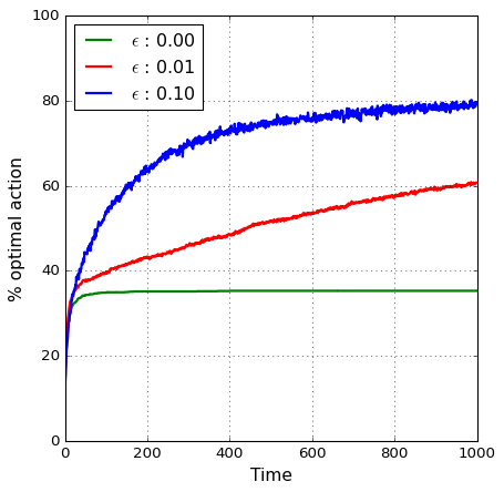
For the case above we investigated a exploration of 10%, but we can do the same simulation for different values of \(\epsilon\). The results can be seen below:

As expected, the pure greedy actions (\(\epsilon = 0\)) does not give a very good average reward in the long run. However, adding some exploration steps looks to improve this.
The more you f*ck around, the more you will find out
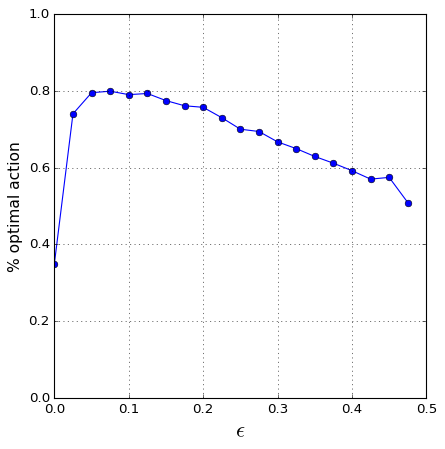
So now for the final question: For this problem, what would be the best \(\epsilon\)? Can we assume that this is true:
To investigate this, simply do several simulations for different values of \(\epsilon\). Then for a certain time, let’s say 1000 steps, investigate the percentage of best actions. Code to do this can look something like this:
values = np.arange(0,0.5,0.025)

Out_vec = []

for va in values:
    # Set up the bandits
    ba = np.zeros(runs)
    bandit = Bandit10(epsilon=va)
    bandit.reset()

    for j in range(runs):
        bandit.reset()

        if j % 500 == 0: print('Iteration: '+str(j))

        for i in range(time):
            action = bandit.getAction()
            bandit.step(action)
        if action == bandit.best_action:
            ba[j] = 1
    Out_vec.append(np.mean(ba))
The result can be seen below:

So the values of 0.1 that was used in the previous example, was actually a good (lucky) guess of an “optimal” \(\epsilon\) value.
Time to conclude
In this first (of hopefully many more) post on the subject of reinforced learning, we had a brief introduction about what separates reinforced learning from other types of learning. We also discussed the balance between exploitation (maximize the reward in the short run) and exploration (may produce a greater total reward in the long run). This was demonstrated by a simple ten armed bandit example.
Well I guess that was all for this time and, as always, feel free to contact us at info@gemello.se