Hi all, time for a new blog post!
To post challenges on different social media platforms is a common thing of today. In this blog post we are going to look at a challenge that was posted way before TikTok and other social media platforms. This one goes back to 1696 and was posted in Acta Eruditorum (which I assume was not as big as the top social media platforms of today) by Johann Bernoulli, a famous Swiss mathematician (one of many prominent mathematicians in the Bernoulli family). He wrote:
I, Johann Bernoulli, address the most brilliant mathematicians in the world. Nothing is more attractive to intelligent people than an honest, challenging problem, whose possible solution will bestow fame and remain as a lasting monument. Following the example set by Pascal, Fermat, etc., I hope to gain the gratitude of the whole scientific community by placing before the finest mathematicians of our time a problem which will test their methods and the strength of their intellect. If someone communicates to me the solution of the proposed problem, I shall publicly declare him worthy of praise
So a bit different introduction than the challenges of today.
Now for the actual challenge. Bernoulli wrote the problem statement as:
Given two points A and B in a vertical plane, what is the curve traced out by a point acted on only by gravity, which starts at A and reaches B in the shortest time.
Ok, the question is quite simple but the solution seems harder… I mean, he did challenge the "most brilliant mathematicians". Since I definitely do not fall into this category I hope that there is something else we can do to find a solution to this problem. To do so, let’s start off by looking at a simpler problem.
Time to simplify
Let’s start to think about a solution by investigating a simpler problem. We need to go back to school where you probably remember that orienteering was part of the syllabus of physical education. You had to run around in the forest with a map where several locations were marked that you had to find. There was also a time aspect so you always wanted to find the way between two marked objects that was the fastest. Now, the picture below shows a very simple map where you start at the top left location (marked with a yellow circle) and you should find the fastest way to the next location at the bottom right (marked by a black circle)
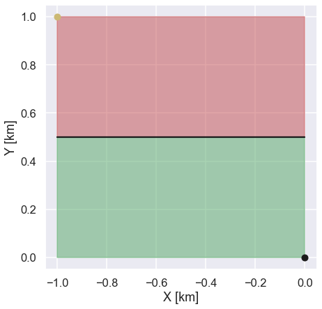
The red area represents the terrain where it is really difficult to run. For the green area, however, the terrain is really nice and flat with no obstacles, so here you can run twice as fast as in the red area. So, if we were to run from the starting point to the end point in the shortest time possible, what path should we take? Well, one idea is to run in a straight line between the starting point and the end point. For sure this is the shortest path possible and it would be the fastest if we could run equally as fast in both the red and the green area. However, since the terrain is much more difficult to access in the red area this might not be the fastest path. A different idea would be to start running the shortest possible distance in the red area, i.e. straight down from the starting point and then when we reach the green area run in a straight line towards the end position. By doing so we spend as little time as possible in the red area where we can not run as fast. However, the total distance we would need to run is much longer than a straight line going directly from the starting point to the end point. So, we somehow need to optimize the relation between speed and distance in order to find the shortest path. Let’s fire up a jupyter notebook and do some coding to find out the fastest path.
Ok, let’s start with some useful imports
import numpy as np
import matplotlib.pyplot as plt
from scipy import interpolate
from scipy.optimize import minimize
import seaborn as sns

sns.set(context='talk')
Since we can run with a constant speed within each area it is a good idea to assume that the fastest way should be made up of two straight lines. One line starts at the black circle in the top left region in the map and and somewhere on the boundary between the red and the green area. The next line continues from the same point on the boundary and goes to the end location on the bottom right. So the question really is to find the point on the boundary between the two different terrains that will give the shortest time. Let’s solve this in the simplest way possible, just try a whole bunch of different points and find which one is the fastest.
v1 = 1
v2 = 2

P1 = np.array([-1,1])
P3 = np.array([0,0])

A = np.linspace(-1,0,10000)
T_vec = []
for a in A:

    P2 = np.array([a,0.5])

    # calculate distance
    ds1 = np.linalg.norm(P1-P2)
    ds2 = np.linalg.norm(P2-P3)

    # calculate time
    dt1 = ds1 / v1
    dt2 = ds2 / v2

    # total time
    t = dt1 + dt2
    T_vec.append(t)

T_vec = np.array(T_vec)

#Find the path with the shortest time and its corresponding location
idx_min = np.argmin(T_vec)
a_min = A[idx_min]
Perhaps not the most sophisticated solution but I think it did the trick. Let’s plot the fastest path and see if there is something interesting about it.
plt.figure(figsize=(7,7))

plt.fill_between([-1,0],[1,1],y2=[0.5,0.5],color='r',alpha=0.5)
plt.fill_between([-1,0],[0.5,0.5],y2=[0.0,0.0],color='g',alpha=0.5)
plt.plot([-1,0],[0.5,0.5],'k')

plt.plot([-1,a_min,0],[1,0.5,0],color='w',lw=3)
plt.plot(-1,1,'yo')
plt.plot(0,0,'ko')
plt.xlabel('X [km]')
plt.ylabel('Y [km]')
plt.show()
and the plot looks like this
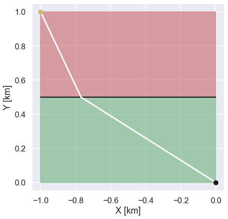
Ok! The shortest path is something in between the two paths that we discussed above. We do not run in a straight line between the starting point and the ending point since we would spend too much time in the area where the terrain is difficult.
So, is there anything particularly interesting with this path? Well what if we look at the angle the path makes in relation to the y-axis (let’s call it \(\phi\)) compared to the speed that you can travel within each area. To be more specific let’s look at the ratio between \(sin(\phi)\) and the speed \(v\)
P2_min = np.array([a_min,0.5])

ds1 = np.linalg.norm(P1-P2_min)
ds2 = np.linalg.norm(P2_min-P3)


sin_fi_1 = (1-np.abs(a_min)) / ds1
sin_fi_2 = np.abs(a_min) / ds2

print('Ratio 1 = ' +str(np.round(sin_fi_1/v1,4)))
print('Ratio 2 = ' +str(np.round(sin_fi_2/v2,4)))
And the results are 0.4191 and 0.4192 respectively. Cool! So the ratio \(sin(\phi) / v \) is constant!
Just to make sure this was not just a funny coincidence let’s do the same thing where we have four different terrains with different maximum speeds. This is shown in the figure below.

The speeds that you can run for each area are, from the top, \(v_1=1\), \(v_2=3\), \(v_3=2\) and \(v_4=0.6\). Ok, a bit more complicated but it should not be that difficult to solve I guess. In this case we are not going to use a brute force solution, instead we are going to use the scipy minimize function. To do so we just need to write a function that calculates the total time it would take to travel a certain path. Since the location of the starting point and the end point is known we only need to find the location on the three different interfaces. Let’s write that function
def calculate_total_time_4(x):

    # speed
    v1 = 1
    v2 = 3
    v3 = 2
    v4 = 0.6

    # path
    x0 = -1.0
    x1 = x[0]
    x2 = x[1]
    x3 = x[2]
    x4 = 0.0

    y0 = 1.0
    y1 = 3/4
    y2 = 2/4
    y3 = 1/4
    y4 = 0.0

    # calcualte distance
    ds1 = np.sqrt( (x0-x1)**2 + (y0-y1)**2)
    ds2 = np.sqrt( (x1-x2)**2 + (y1-y2)**2)
    ds3 = np.sqrt( (x2-x3)**2 + (y2-y3)**2)
    ds4 = np.sqrt( (x3-x4)**2 + (y3-y4)**2)

    #calcualte time
    t1 = ds1 / v1
    t2 = ds2 / v2
    t3 = ds3 / v3
    t4 = ds4 / v4

    return t1+t2+t3+t4
Nice, not that complicated. Now, we simply use the minimize function to find the fastest path
res = minimize(calculate_total_time_4, [-0.8,-0.5,-0.2],method='BFGS' )
That was easy. Finally we plot the path.
x0 = -1.0
x1 = res.x[0]
x2 = res.x[1]
x3 = res.x[2]
x4 = 0.0

y0 = 1.0
y1 = 3/4
y2 = 2/4
y3 = 1/4
y4 = 0.0


plt.figure(figsize=(7,7))

plt.fill_between([-1,0],[y0,y0],y2=[y1,y1],color='r',alpha=0.5)
plt.fill_between([-1,0],[y1,y1],y2=[y2,y2],color='b',alpha=0.5)
plt.fill_between([-1,0],[y2,y2],y2=[y3,y3],color='g',alpha=0.5)
plt.fill_between([-1,0],[y3,y3],y2=[y4,y4],color='y',alpha=0.5)

plt.plot([-1,0],[y1,y1],'k')
plt.plot([-1,0],[y2,y2],'k')
plt.plot([-1,0],[y3,y3],'k')

#plt.plot([x0,x1,x2,x3,x4],[y0,y1,y2,y3,y4],color='w',lw=3)
plt.plot(-1,1,'yo')
plt.plot(0,0,'ko')
plt.xlabel('X [km]')
plt.ylabel('Y [km]')
plt.show()
Giving the following figure
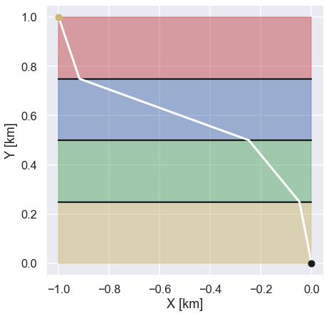
Nice! This seems like a good solution since we travel the shortest distance in the terrain where we have the lowest speed. Just to finish this exercise let’s look at the ratios between the angles of the path and the speed for each terrain.
v1 = 1
v2 = 3
v3 = 2
v4 = 0.6


ds1 = np.sqrt( (x1-x0)**2 + (y1-y0)**2 )
sin_fi_1 = (x1-x0)/ds1

ds2 = np.sqrt( (x2-x1)**2 + (y2-y1)**2 )
sin_fi_2 = (x2-x1)/ds2

ds3 = np.sqrt( (x3-x2)**2 + (y3-y2)**2 )
sin_fi_3 = (x3-x2)/ds3

ds4 = np.sqrt( (x4-x3)**2 + (y4-y3)**2 )
sin_fi_4 = (x4-x3)/ds4


print('Ratio 1 = ' +str(np.round(sin_fi_1/v1,4)))
print('Ratio 2 = ' +str(np.round(sin_fi_2/v2,4)))
print('Ratio 3 = ' +str(np.round(sin_fi_3/v3,4)))
print('Ratio 4 = ' +str(np.round(sin_fi_4/v4,4)))
and what do you know, that all turned out to be 0.3123. Super nice!
We have now made it credible that if we should find the fastest path between to different locations the relation between the direction we travel,the angle, and the speed that we can travel is always constant. To put this is math:
$$\dfrac{sin(\phi)}{v}=C$$Well, I think that I have seen this relationship between the angle and the speed before… Yes, going back to physics class in school we learned that the refraction of light at the interface between two different media (different speeds) follow the same relationship. This basically means that light does the thing that we are interested in which is summarized in Fermat's principle
Fermat’s principle: If a beam of light travels between from point A to B, it does so along the fastest path possible.
Alright! I think that we are ready to look at the original problem!
This is the (fastest) way
So, ones again, the problem was stated like this by Johann Bernoulli:
Given two points A and B in a vertical plane, what is the curve traced out by a point acted on only by gravity, which starts at A and reaches B in the shortest time.
From the above we have found out that we should follow the light in order to find the solution. This is what Johann Bernoulli used in order to solve the problem back in 1696 way before computers and jupyter notebooks (must have been difficult…). Just in order for us to do some calculations let’s define the two points A and B in the problem formulation above according to the picture below.
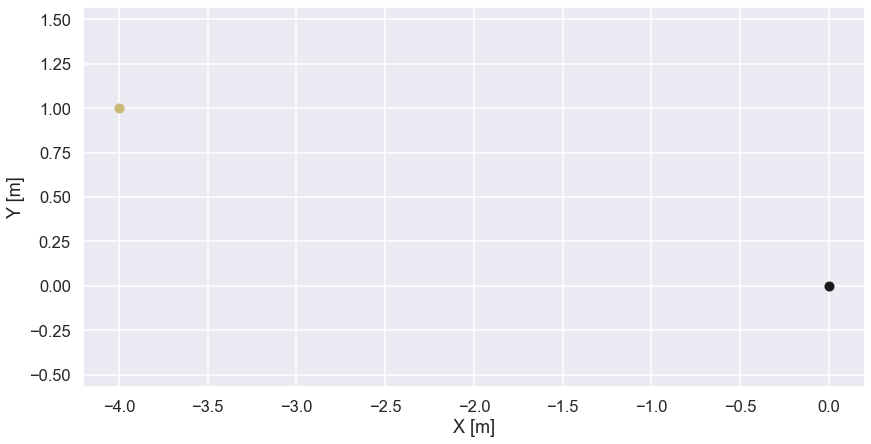
Note that this is the vertical plane so gravity acts along the negative y-axis.
We know that the ratio \(sin(\psi) / v \) is constant but how do we calculate the speed? This is actually quite easy since we are allowed to use conservation of energy (no losses due to friction or air resistance and so on). This means that the change in potential energy equals the change in kinetic energy which gives us the following expression for the speed.
$$v=\sqrt{2gh}$$
where \(g\) is the gravitational acceleration and \(h\) is the distance the “point” has dropped from its starting position. To make a plot similar to the ones we looked at above (the orienteering maps) we make a scatter plot of the speed.
X_scatter_speed = []
Y_scatter_speed = []
V_scatter_speed = []


for xx in np.linspace(-4,0,400):
    for yy in np.linspace(-0.5,1.0,100):
        X_scatter_speed.append(xx)
        Y_scatter_speed.append(yy)
        V_scatter_speed.append(np.sqrt(2*9.81*(1-yy)))


plt.figure(figsize=(14,7))

plt.scatter(X_scatter_speed,Y_scatter_speed,c=V_scatter_speed,s=10,cmap='magma')
plt.plot(-4,1,'yo')
plt.plot(0,0,'ko')

plt.colorbar()

plt.axis('equal')
plt.xlabel('X [m]')
plt.ylabel('Y [m]')
plt.show()
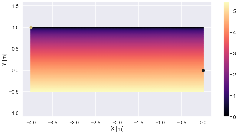
Nice! Now we know how the speed changes as a function of the y-coordinate so we should be able to find the path with the shortest time. For sure there is a nice analytical solution to this problem, see here for instance, but we are going to use a much simpler method.
- Start at some angle and speed
- Take a really small step in this direction
- At the end of the step calculate the new speed
- Update the angle according to \(sin(\psi) / v = C \)
- Goto 2 and repeat until we have reached the end point
For sure we need to adjust the constant \(C\) so we reach the end point (black point in figure above). Below the code for this procedure is shown.
sin_fi = 0 * np.pi/180
d_step = 0.01
C = 0.184

X_optimum = []
Y_optimum = []

P_x = -4
P_y = 1

X_optimum.append(P_x)
Y_optimum.append(P_y)

keep_on_going = True
passed_low_point = False

while keep_on_going:

    if passed_low_point:
        P_x = P_x +sin_fi*d_step
        P_y = P_y + np.sqrt(1-sin_fi**2)*d_step
    else:
        P_x = P_x +sin_fi*d_step
        P_y = P_y - np.sqrt(1-sin_fi**2)*d_step
    X_optimum.append(P_x)
    Y_optimum.append(P_y)
    v = np.sqrt(2*9.81*(1-P_y))
    #print(sin_fi)
    sin_fi = C * v
    if sin_fi>1.0:
        sin_fi = 2-sin_fi
        passed_low_point = True

    if P_x > 0.0:
        keep_on_going = False
Note that there is a “fix” if the path switches from a descending to an ascending direction. Here is a plot of the path.
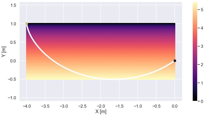
Allright! That looks kind of interesting. Starting off kind of steep and then curves in some sort of arc. It is also interesting to see that the path is passing below the level of the end point in order to move at the highest possible speed.
Just as a “grand finale” let's compare the time it takes to reach the end position for the three different paths shown below (the green one is the optimized path that we just calculated)
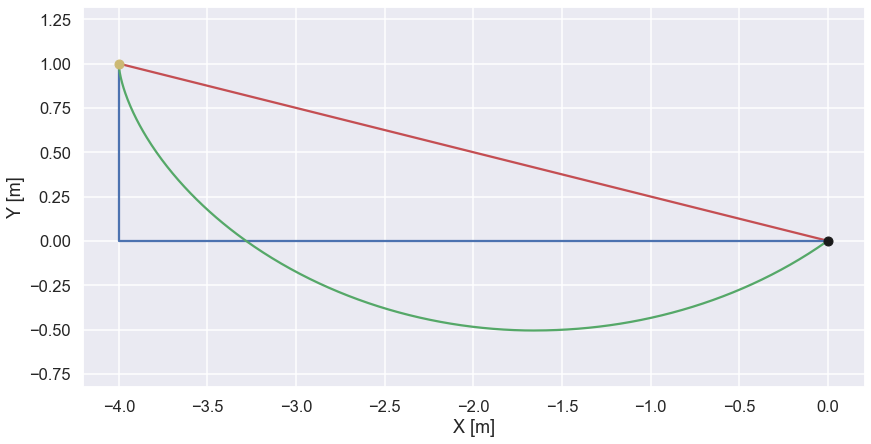
The two other paths are stored in a similar format as the optimized paths.
X_linear = np.linspace(-4,0,500)
Y_linear = -1/4*X_linear

X_vertical = np.concatenate([np.ones(100)*-4,np.linspace(-4,0,400)])
Y_vertical = np.concatenate([np.linspace(1,0,100),np.zeros(400)])
To calculate the time we define a function that returns an array with the time corresponding to each position of the path
def time_for_path(x,y):

    t_vec = []
    t = 0
    t_vec.append(t)

    g = 9.81


    # --- calculate time
    for i in range(1,len(x)):
        x_old = x[i-1]
        y_old = y[i-1]
        v_old = np.sqrt(2*g*(y[0]-y_old))

        x_new = x[i]
        y_new = y[i]
        v_new = np.sqrt(2*g*(y[0]-y_new))

        ds = np.sqrt((x_new-x_old)**2+(y_new-y_old)**2)
        v_avg = (v_old + v_new)/2
        dt = ds/v_avg
        t = t + dt
        t_vec.append(t)


    return t_vec
Not too complicated I would say. Now the total time for the optimized path is calculated as
t_vec_optimum = time_for_path(X_optimum,Y_optimum)
t_vec_optimum[-1]
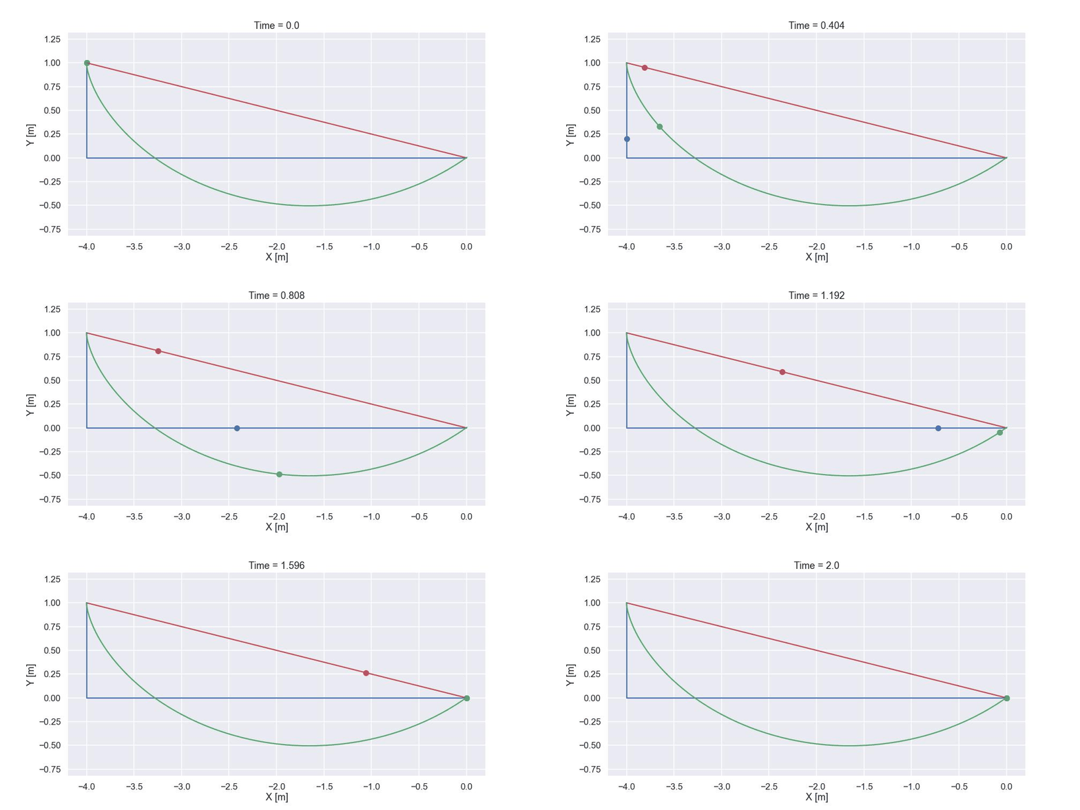
and the result was 1.213 sec. The time for the shortest path is calculated in a similar way and the time was 1.861 sec. For the path that starts with a vertical drop and then continuous horizontally towards the end point the time was 1.354 sec. So the optimized path indeed is the fastest path (at least out of the one tested...). For sure we must have an animation of the three different paths and here it comes!
Time to conclude
That was it for this blog post! I think we managed to find an acceptable solution to this very famous problem. Using python we really did not have to flex any mathematical muscles which is super convenient since the ones I have are really small.
Well I guess that was all for this time and, as always, feel free to contact us at info@gemello.se