Hi all, time for a new blog post!
This will be a blog post similar to probably a gazillion other blog posts you can find online: Neural Network from Scratch in Python. (It will actually not be "from scratch" we will use Numpy to simplify things...)
It starts with some data
In this blog post we are going to look at a classification problem i.e. we should determine which “class” a certain data point belongs to. To do so we have a sort of toy example as shown below.
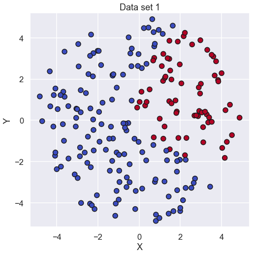
So, each data point has an X value and a Y value and each data point can belong to one out of two classes. The data is stored as an \( \mathbf{X} \) matrix where each data point makes up a column in \( \mathbf{X} \) so the shape of the matrix is (2,207) (since there are 207 datapoints). The class of each data point is stored in an array called \( \mathbf{y} \) where the specific class is represented by the integer 0 or 1.
Now that we have some data let’s start with the building of a model that could predict the class of any data point. We will use the data set we have to “train” the model to identify the class of the new data point given its two input values. Let’s start to look at an artificial neural network and how it is constructed.
So, what is a Neural Network?
The Idea of an artificial neural network is a model inspired by the structure and function of biological neural networks in animal brains. A sketch of the neural network that we are going to use in this blog post is given below.
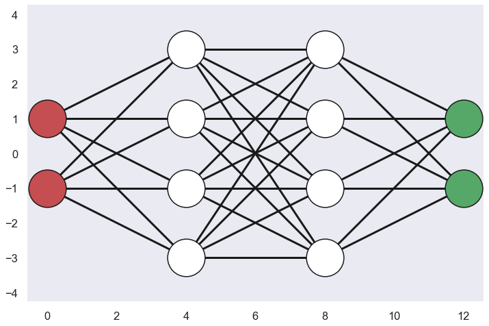
What is this then?? Each circle in the network above is called a neuron since the idea is that they “loosely” model the neurons in a brain. There are several layers of neurons in a neural network and if we start to the left with the two red neurons they represent the input layer of the network. There are two of them since they represent the two input parameters of the model, the X and Y values.
Going to the other end of the network we have the two green neurons which represent the output layer of the network. Here we also have two neurons and the reason for this is that the data points can belong to two different classes, i.e. each neuron represents each class
The white nodes in the middle of the network represent hidden layers and in this network we have two hidden layers with four neurons in each layer. This number of hidden layers and the size of each hidden layer is here chosen a bit arbitrary and we will not go into the question on what shape of the neural network to choose in this blog post.
As can be seen from the sketch above each neuron in a layer is connected to all the neurons in the previous layer i.e. all neurons in the previous layer acts as input to a specific neuron in the current layer. Likewise, the output of a specific neuron in the current layer will act as inputs to all the neurons in the next layer. The connections are often referred to as edges.
Let’s look at what happens when data is passed forward in the neural network from the input layer to the output layer.
I take two steps forward...
So, let’s look at the “mechanics” of a neural network. The first thing we need to do is to say something about the notation. Since the neural network has several layers and each layer has several neurons we need some simple notation to understand how things are related to each other. A super script will refer to a specific layer e.g. the vector \( \mathbf{a}^2 \) refers to the output from layer 2. If we look at a specific component of this vector e.g. \( a^2_3 \) we refer to the output of the third neuron in the second layer. Now, let’s look at an arbitrary neuron in an arbitrary layer.
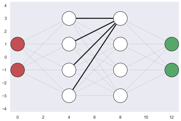
So the arbitrary neuron turned out to be the first neuron in the second hidden layer. As can be seen from the sketch this neuron is connected with all the neurons in the previous layer. Now, the input to this neuron can be written as a weighted sum of all the outputs from the previous layer and some bias, this is written as.
\[ z^2_1 = W^2_{11} \cdot a^1_1 + W^2_{12} \cdot a^1_2 + W^2_{13} \cdot a^1_3 + W^2_{14} \cdot a^1_4 + b^2_1 \]
Perhaps a note on the notation. \( z^2_1 \) denotes the input to the first neuron in the second hidden layer (the first layer has index 0 ) and the components \(a^1_1, a^1_2, a^1_3,\) and \(a^1_4\) are the output from the previous layer. Now, what is then \(W^2_{11}, W^2_{12}, W^2_{13} \) and \( W^2_{14} \) ? These are weight that modify the outputs from each of the neurons in the previous layer before they are summed up. Moreover, the bias \( b^2_1 \) is added on top of this to form the input the studied neuron. Note that for the moment we do not know the values of the weights and the bias, and we will spend a lot of time on how to determine these values in subsequent sections.
Now, we have the value that is entering the neuron, what about the output from the neuron? Well, we could just leave it as it is i.e. just using the weighted sum as output, but this limit our possibilities to use the neural network to model something exciting. It turns out that for this option we will only have a linear model no matter how many layers of neurons we add…
So we need something else… an activation function.
It would be nice if this function could be really simple but still be used to describe something non-linear. Let’s look at the Rectified Linear Unit or ReLU function.
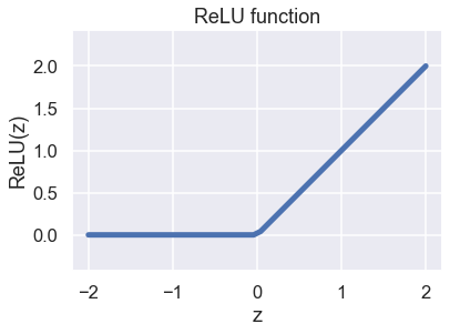
If the input value is greater than 0 then the output value is simply the same as the input value but incase that the input is negative it just returns 0. Something like this
\[ ReLU(z) = max(0,z) \]
Nice, not that complicated and clearly non-linear. Using this activation function the output from the first neuron in the second hidden layer would look like this:
\[ a^2_1 = ReLU(z^2_1) \]
Sweet! We have now by just two equations related the outputs from all the neurons in a previous layer to the output of a specific neuron in the current layer. Let’s do the same thing for the second neuron in the same layer.
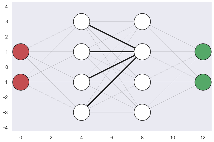
So, the weighted sum would look like this:
\[ z^2_2 = W^2_{21} \cdot a^1_1 + W^2_{22} \cdot a^1_2 + W^2_{23} \cdot a^1_3 + W^2_{24} \cdot a^1_4 + b^2_2 \]
Note that the weights and the bias are not the same as previous i.e. they will be unique for each neuron. Moreover, the by applying the ReLU activation function we get the output from this neuron.
\[ a^2_2 = ReLU(z^2_2) \]
So, very similar to what is going on for the first neuron in this layer.
Let’s try to make a summary of what we have done. Returning to the expression for the weighted sum, we can use matrix multiplication to get something like this:
\[ \begin{bmatrix} z^2_{1} \\ z^2_{2} \end{bmatrix} = \begin{bmatrix} W^2_{11} & W^2_{12} & W^2_{13} & W^2_{14} \\ W^2_{21} & W^2_{22} & W^2_{23} & W^2_{24} \\ \end{bmatrix} \cdot \begin{bmatrix} a^1_{1} \\ a^1_{2} \\ a^1_{3} \\ a^1_{4} \end{bmatrix} + \begin{bmatrix} b^2_{1} \\ b^2_{2} \end{bmatrix} \]
Nice! You would not need that much imagination to come up with the expression for the two remaining neurons in this layer... It would look like this
\[ \begin{bmatrix} z^2_{1} \\ z^2_{2} \\ z^2_{3} \\ z^2_{4} \end{bmatrix} = \begin{bmatrix} W^2_{11} & W^2_{12} & W^2_{13} & W^2_{14} \\ W^2_{21} & W^2_{22} & W^2_{23} & W^2_{24} \\ W^2_{31} & W^2_{32} & W^2_{33} & W^2_{34} \\ W^2_{41} & W^2_{42} & W^2_{43} & W^2_{44} \\ \end{bmatrix} \cdot \begin{bmatrix} a^1_{1} \\ a^1_{2} \\ a^1_{3} \\ a^1_{4} \end{bmatrix} + \begin{bmatrix} b^2_{1} \\ b^2_{2} \\ b^2_{3} \\ b^2_{4} \end{bmatrix} \]
or, written more compact like
\[ \mathbf{z}^2 = \mathbf{W}^2 \cdot \mathbf{a}^1 + \mathbf{b}^2 \]
So, we can easily propagate the output from one layer to input to the next layer by using this nice compact formula.
Now that the we have the input to the entire layer we can apply the activation function to the whole vector in order to obtain the output from this layer. In case of the ReLU activations function we can write it like this
\[ \mathbf{a}^2 = ReLU(\mathbf{z}^2) \\ \]
Where we simply apply the ReLU function to each component of the vector. So, the thing that will happen when we pass information forward in the network, i.e. going from the very first input layer to the hidden layers and finally ending up at the output layer, can be described by a calculation of the weighted sum and a subsequent activation function.
\[ \begin{split} \mathbf{z}^l &= \mathbf{W}^l \cdot \mathbf{a}^{l-1} + \mathbf{b}^l \\ \mathbf{a}^l &= f(\mathbf{z}^l) \\ \end{split} \]
Where \(f\) indicates some sort of activation function.
Before we wrap up this section, let's look at the activation function for the output layer. The output layer has two neurons that represents the two possible classes that the data point can have, in this toy example the value 1 or 0. So, a really nice feature would be if the output would be interpreted as some sort of probability of one or the other class. Well, today is our lucky day becourse this property can be found in the SoftMax activation function which is defined as:
\[ \mathbf{a}^3 = SoftMax(\mathbf{z}^3) = \frac{e^{\mathbf{z}^3}}{\sum_i e^{z^3_i}} \\ \]
This function will garantie that the output from each neuron will be non-negative and the sum of the output for all neurons will be equal to 1 i.e. the things that you would expect from a probability distribution function, nice!
I think that we have everything covered when it comes to passing data forward through the neural network, nice!! Just to be clear, let's just make a small summary before we continue to the next section. Starting with the input \( \mathbf{a}^0 \) and ending with the output \( \mathbf{a}^3 \).
\[ \begin{split} \mathbf{z}^1 &= \mathbf{W}^1 \cdot \mathbf{a}^0 + \mathbf{b}^1 \\ \mathbf{a}^1 &= ReLU(\mathbf{z}^1) \\ \mathbf{z}^2 &= \mathbf{W}^2 \cdot \mathbf{a}^1 + \mathbf{b}^2 \\ \mathbf{a}^2 &= ReLU(\mathbf{z}^2) \\ \mathbf{z}^3 &= \mathbf{W}^3 \cdot \mathbf{a}^2 + \mathbf{b}^3 \\ \mathbf{a}^3 &= SoftMax(\mathbf{z}^3) \\ \end{split} \]
What is the Cost?
We have now looked at the “mechanics” of the neural network and it turned out that we can propagate information from the input layer all the way to the output layer by passing information layer by layer using two simple equations.
Nice, really simple.
The problem, however, what vales should all the different weight and biases have? Just to clear, there are a lot of different weight and biases that somehow needs to be determined. Here comes the idea that we can learn from the data set that we looked at in the beginning of this post. We can send in the \(X\) and \(Y\) value of a specific data point into the neural network and compare the output we get, a probability of which class this data point will belong to, to the actual class. For sure, the value of the different weights and biases will affect how good the prediction will be. So, what we need is some function that will give us a number that tells us how “good” the prediction is when compared to the actual class.
This function is often referred to as the loss function. There are several options but in this post we will use the Cross Entropy Loss function and has the following form
\[ C(\mathbf{y},\mathbf{a}^3) = -\sum_i y_i \log(a^3_i) \]
Where the vector \(\mathbf{y}\) represents the actual class of the data point and \(\mathbf{a}^3\) is the output from the neural network.
Here a small modification to the \(\mathbf{y}\) vector is done so it will be easier to compare it to the output of the neural network. We have used what is called one hot encoding where the representation of the class is represented by two digits. The probability of the data point belonging to class 0 and the probability that the data point belongs to class 1. By doing this we get the actual data in the same format as the prediction from the neural network.
Let’s just look at an example to get some sort of feeling for this loss function (to be honest, it is probably not clear that will form will works as a loss function). If the current data point belongs to category 1 the one hot encoding would look like \( \mathbf{y} = [0,1] \) and let’s say that the prediction from the neural network looks like \( \mathbf{a}^3 = [0.367,0.633] \). Note that the sum of the output is equal to 1 since we used the SoftMax activations function for the output layer. If we use the equation above for the cross entropy loss function we would get the following:
\[ C = -y_1 log(a^3_1) – y_2 log(a^3_2) = -0\cdot log(0.367) – 1 \cdot log(0.633) = -log(0.633) \]
Since we use one hot encoding for the data only one term of the sum will be non-zero. Moreover, we would like the component of \( \mathbf{a}^3 \) for this remaining term to be as close to 1 as possible (since this would mean that we are very certain about the correct answer) and this would minimize the cost function. Just to increase the understanding of the cost function even more we can plot the cost function for the same value of the data i.e. \( \mathbf{y} = [0,1] \) for different values of the output i.e. \( \mathbf{a}^3 = [1-a,a] \).
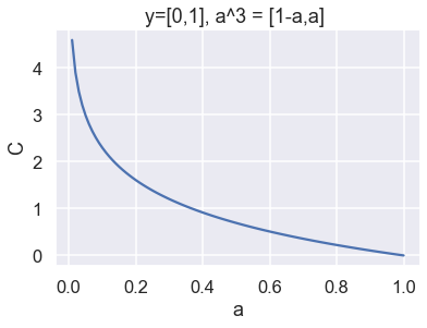
Nice! As can be seen, the value of the cost function decreases toward 0 as the output vector gets closer to the true value of the data.
To get the cost function for all the data points we just sum the cost for each data point. So we now have a function that can tell us something about how good the prediction of the neural network is when compared to a known data set and we can now turn our interest towards the really important question that we sort of overlooked so far…. What should the values be for all the weights as biases be???
Since we have defined a cost function, we can easily compare two different setups of all the weights and biases and say which one is the best but there must be a way to calculate how we should change the weights and biases in order for the cost function to decrease…
As you can see this has turned into an optimization problem where the aim is to minimize the cost function and the things that we can change in order to do so are the different weights and biases. So there is nothing magical with the term “training the neural network”, the only thing we are trying to do is to minimize the difference between the thing predicted by the neural network and the actual data. So basically, we could use any sort of optimization algorithm in order to find the “best” values of the weight and the biases and in this blog post we will be using the gradient descent method.
The concept of gradient descent method is quite intuitive. The idea is to take repeated steps in the opposite direction of the gradient (or approximate gradient) of the function at the current point, because this is the direction of steepest descent. Written in some math it could look something like this (for the weight \( \mathbf{W}^3 \) ):
\[ (\mathbf{W}^3)^{n+1} = (\mathbf{W}^3)^n - \gamma \frac{\partial C}{\partial \mathbf{W}^3} \]
Here the \( \gamma \) thing is called learning rate and is basically a step size. Similar expressions are used for all the other weights and biases.
Alright we now have a cost function and a method to update our different weights and biases in order to minimize this cost function, we should be ready to now. Well, yes, we are apart from that this gradient thing seems quite difficult to calculate… I mean this cost function is a non-linear function of a non-linear function of a non-linear function….. So, let’s spend the next section on this topic where the concept of backpropagation is described.
I take two steps back...
Just as a warning, this will be a bit heavy on math stuff, but have no fear I think it will work out fine any way
So, we would like to calculate the gradient of the cost function in order to update our weights and biases and due to the structure of the neural network we are going to go completely bananas with the chain rule when calculating the gradients so let’s start with what the chain rule is.
A short description of the chain rule from Wikipedia: If a variable z depends on the variable y, which itself depends on the variable x (that is, y and z are dependent variables), then z depends on x as well, via the intermediate variable y. In this case, the chain rule is expressed as
\[ \frac{dz}{dx} = \frac{dz}{dy} \frac{dy}{dx} \]
Not that complicated, but keep in mind that this could go on more or less forever if there are many variables that are functions of other variables that are functions of other variables…. Perhaps the easiest way is just to start with calculating the gradient of the cost function with respect the weight \( \mathbf{W}^3 \) and just see what will happen…
The cost function is a function of the output from the last layer of the neural network \( \mathbf{a}^3 \) which is a function of the input to the last layer, \( \mathbf{z}^3 \), this via the SoftMax activation function. Finally the variable \( \mathbf{z}^3 \) is a function of the weight \( \mathbf{W}^3 \) so if we use the chain rule it could look something like this:
\[ \frac{\partial C}{\partial \mathbf{W}^3} = \frac{\partial C}{\partial \mathbf{a}^3} \cdot \frac{\partial \mathbf{a}^3}{\partial \mathbf{z}^3} \cdot \frac{\partial \mathbf{z}^3}{\partial \mathbf{W}^3} \]
The first two terms in the expression are a bit tedious to evaluate so we will just state the results and if you are interested in how this is calculated you can check out this webpage. Let’s include the this in the expression above as well as evaluate the final term.
\[ \frac{\partial C}{\partial \mathbf{W}^3} = (\mathbf{a}^3 - \mathbf{y} ) \cdot \frac{\partial \mathbf{z}^3}{\partial \mathbf{W}^3} = (\mathbf{a}^3 - \mathbf{y} ) \cdot \frac{\partial \mathbf{W}^3 \cdot \mathbf{a}^2 + \mathbf{b}^3 }{\partial \mathbf{W}^3} = \mathbf{\delta}^3 \cdot (\mathbf{a}^2)^T \]
Here we have defined the “error” for the output layer as \( \mathbf{\delta}^3 = (\mathbf{a}^3 - \mathbf{y}) \) and the \( (*)^T \) represents the transpose of the vector. So, we have arrived at a very compact and simple expression for the gradient of the cost function with respect to \( \mathbf{W}^3 \). Let’s see what happens when we calculate the gradient with respect to \( \mathbf{b}^3 \).
\[ \frac{\partial C}{\partial \mathbf{b}^3} = (\mathbf{a}^3 - \mathbf{y} ) \cdot \frac{\partial \mathbf{z}^3}{\partial \mathbf{b}^3} = (\mathbf{a}^3 - \mathbf{y} ) \cdot \frac{\partial \mathbf{W}^3 \cdot \mathbf{a}^2 + \mathbf{b}^3 }{\partial \mathbf{b}^3} = \mathbf{\delta}^3 \]
Sweet! Even more compact and simple. We have now calculated the gradient with respect the weight and bias connected to the input of the last layer in the neural network. Let’s continue backwards in the network and see what will happen when we calculate the gradient with respect to the weight \( \mathbf{W}^2 \).
\[ \begin{split} \frac{\partial C}{\partial \mathbf{W}^2} &= \mathbf{\delta}^3 \cdot \frac{\partial \mathbf{W}^3 \cdot \mathbf{a}^2 + \mathbf{b}^3 }{\partial \mathbf{W}^2} = \mathbf{\delta}^3 \cdot \mathbf{W}^3 \cdot \frac{\partial \mathbf{a}^2 }{\partial \mathbf{W}^2} \\ & = \mathbf{\delta}^3 \cdot \mathbf{W}^3 \cdot \frac{\partial \mathbf{a}^2}{\partial \mathbf{z}^2} \cdot \frac{\partial \mathbf{z}^2}{\partial \mathbf{W}^2} \\ & = \mathbf{\delta}^3 \cdot \mathbf{W}^3 \cdot \frac{\partial ReLU(\mathbf{z}^2)}{\partial \mathbf{z}^2} \cdot \frac{\partial \mathbf{W}^2 \cdot \mathbf{a}^1 + \mathbf{b}^2}{\partial \mathbf{W}^2 } \end{split} \]
So, the last term we have sort of seen before, we are just in a different layer compared to last time. The derivative of the ReLU function with respect to \( \mathbf{z}^2 \) should be quite ok to calculate, it is an square matrix with the term \( ReLU’(z^2_i) \) in the diagonal. . After some small rearrangement of the above equations we finally get
\[ \begin{split} \frac{\partial C}{\partial \mathbf{W}^2} &= (\mathbf{W}^3)^T \cdot \mathbf{\delta}^3 \odot ReLU'(\mathbf{z}^2) \cdot (\mathbf{a}^1)^T \\ & = \mathbf{\delta}^2 \cdot (\mathbf{a}^1)^T \end{split} \]Where \( \odot \) is the Hadamard product which is the same as multiplication of to arrays in python. Now we see something cool, we can “propagate” the error \(\mathbf{\delta}^3 \) backwards to the previous layer by using this formula.
\[ \mathbf{\delta}^{2} = (\mathbf{W}^3)^T \cdot \mathbf{\delta}^3 \odot ReLU'(\mathbf{z}^{2}) \]
Then we can calculate the gradients with respect of \( \mathbf{W}^2 \) and \( \mathbf{b}^2 \) with this simple relations
\[ \begin{split} \frac{\partial C}{\partial \mathbf{W}^2} &= \mathbf{\delta}^2 \cdot (\mathbf{a}^1)^T \\ \frac{\partial C}{\partial \mathbf{b}^2} &= \mathbf{\delta}^2 \end{split} \]
Really nice! By similar calculations as above we can calculate the gradients with respect to \( \mathbf{W}^1 \) and \( \mathbf{b}^1 \)
\[ \begin{split} \mathbf{\delta}^{1} &= (\mathbf{W}^2)^T \cdot \mathbf{\delta}^2 \odot ReLU'(\mathbf{z}^{1}) \\ \frac{\partial C}{\partial \mathbf{W}^1} &= \mathbf{\delta}^1 \cdot (\mathbf{a}^0)^T \\ \frac{\partial C}{\partial \mathbf{b}^1} &= \mathbf{\delta}^1 \end{split} \]
Believe if or not but we have now calculated the gradients of all the weights and biases so basically, we can start training the network. Just one more thing regarding the gradients. The relations above are calculated for one data point at a time so to get the “total” gradients we just calculate an average of many data points.
Now, let’s do some coding!!
Make it work
Let’s just have a look at the data one more time.

We have just over 200 data points where some belongs to the 0 category and some belongs to the 1 category.
Let's just change the format of information of the category to the one hot encoding format
a0_train = np.zeros((2,len(idx_train)))
a0_train[0,:] = X_train
a0_train[1,:] = Y_train


one_hot_encoding = np.zeros((2,len(idx_train)))
one_hot_encoding[0,:] = 1-idx_train
one_hot_encoding[1,:] = idx_train
Where the variable idx_train holds the category of each data point i.e. 0 or 1. Now the code that does all the work
# some stuff just for plotting
C_func_array = []
Parameter_list = []


# learning rate
LR = 0.2

# Set input data
a0 = a0_train
y = one_hot_encoding


# Initiate weights and biasis
W1 = np.random.random(size =(4,2)) - 0.5
b1 = np.random.random(size=(4,1)) - 0.5

W2 = np.random.random(size =(4,4)) - 0.5
b2 = np.random.random(size=(4,1)) - 0.5

W3 = np.random.random(size =(2,4)) - 0.5
b3 = np.random.random(size=(2,1)) - 0.5


for _ in range(0,1000):

    # ----- Feed Forward -----

    # 1st layer
    z1 = W1.dot(a0) + b1
    a1 = np.maximum(z1,0)  # ReLU

    # 2nd layer
    z2 = W2.dot(a1) + b2
    a2 = np.maximum(z2,0)  # ReLU

    # 3rd layer, Output
    z3 = W3.dot(a2) + b3
    a3 = np.exp(z3) / np.sum(np.exp(z3),axis=0)  # Soft Max

    # Cost function
    Cost_function = - np.sum(y * np.log(a3)) # Cross-entropy

    # Just for plotting
    C_func_array.append(Cost_function)
    Parameter_list.append( [W1,b1,W2,b2,W3,b3])

    # ----- Back Propagation ------

    # initiate grad
    dC_dW3 = np.zeros(np.shape(W3))
    dC_dW2 = np.zeros(np.shape(W2))
    dC_dW1 = np.zeros(np.shape(W1))

    dC_db3 = np.zeros(np.shape(b3))
    dC_db2 = np.zeros(np.shape(b2))
    dC_db1 = np.zeros(np.shape(b1))

    # random datapoints for evaluation
    m = 100
    idx_grad = np.random.randint(low=0,high=y_batch.shape[1],size=m)

    # calculate grad
    for i in idx_grad:

        # propagate error backwards
        delta3 = (a3[:,i:i+1]-y[:,i:i+1])
        delta2 = W3.T.dot(delta3) * ReLU_prim(z2[:,i:i+1])
        delta1 = W2.T.dot(delta2) * ReLU_prim(z1[:,i:i+1])

        dC_dW3 = dC_dW3 + delta3 * a2[:,i:i+1].T
        dC_dW2 = dC_dW2 + delta2 * a1[:,i:i+1].T
        dC_dW1 = dC_dW1 + delta1 * a0[:,i:i+1].T

        dC_db3 = dC_db3 + delta3
        dC_db2 = dC_db2 + delta2
        dC_db1 = dC_db1 + delta1

    # --- update weight and bias
    W1 = W1 - LR*dC_dW1/m
    W2 = W2 - LR*dC_dW2/m
    W3 = W3 - LR*dC_dW3/m

    b1 = b1 - LR*dC_db1/m
    b2 = b2 - LR*dC_db2/m
    b3 = b3 - LR*dC_db3/m
Nice! not that much code I think. The first thing we can look at is perhaps if the neural network has learned anything during the training. To do this let's plot the cost function for each iteration and hopefully this has decreased dramatically during the training.
plt.figure(figsize=(8,6))
plt.plot(C_func_array,lw=3)
plt.xlabel('Iterations')
plt.ylabel('Error function')
plt.title('Error function')
plt.show()
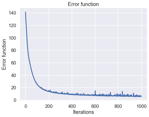
This looks rater good I would say. There is a huge improvement during the say first 200 iterations and then the improvements are a bit slower. This is in line with the general performance of a steepest descent algorithm where the step size is small near the good solusion.
Let's continue to the final solution and see what kind of prediction this trained neural network would give
ii = 999

W1 = Parameter_list[ii][0]
b1 = Parameter_list[ii][1]
W2 = Parameter_list[ii][2]
b2 = Parameter_list[ii][3]
W3 = Parameter_list[ii][4]
b3 = Parameter_list[ii][5]

# Feed Forward
# 1st layer
z1 = W1.dot(a_plot) + b1
a1 = np.maximum(z1,0)  # ReLU

# 2nd layer
z2 = W2.dot(a1) + b2
a2 = np.maximum(z2,0)  # ReLU

# 3rd layer, Output
z3 = W3.dot(a2) + b3
a3_plot = np.exp(z3) / np.sum(np.exp(z3),axis=0)  # Soft Max


plt.figure(figsize=(10,8))
plt.scatter(a_plot_X,a_plot_Y,c=a3_plot[1,:],cmap='coolwarm',s=2)
plt.scatter(X_train,Y_train,c=idx_train_2,cmap='coolwarm',edgecolor='k',s=100)
plt.axis('equal')

plt.xlabel('X')
plt.ylabel('Y')
plt.title('Data set 1')
plt.show()
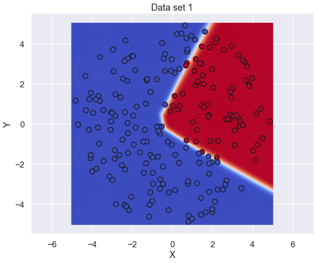
Really nice! There is a small boundary where the neural network is not certain about the category but overall perforamnce seams to be very good.
For sure we need an animation of how the network will perform during the training
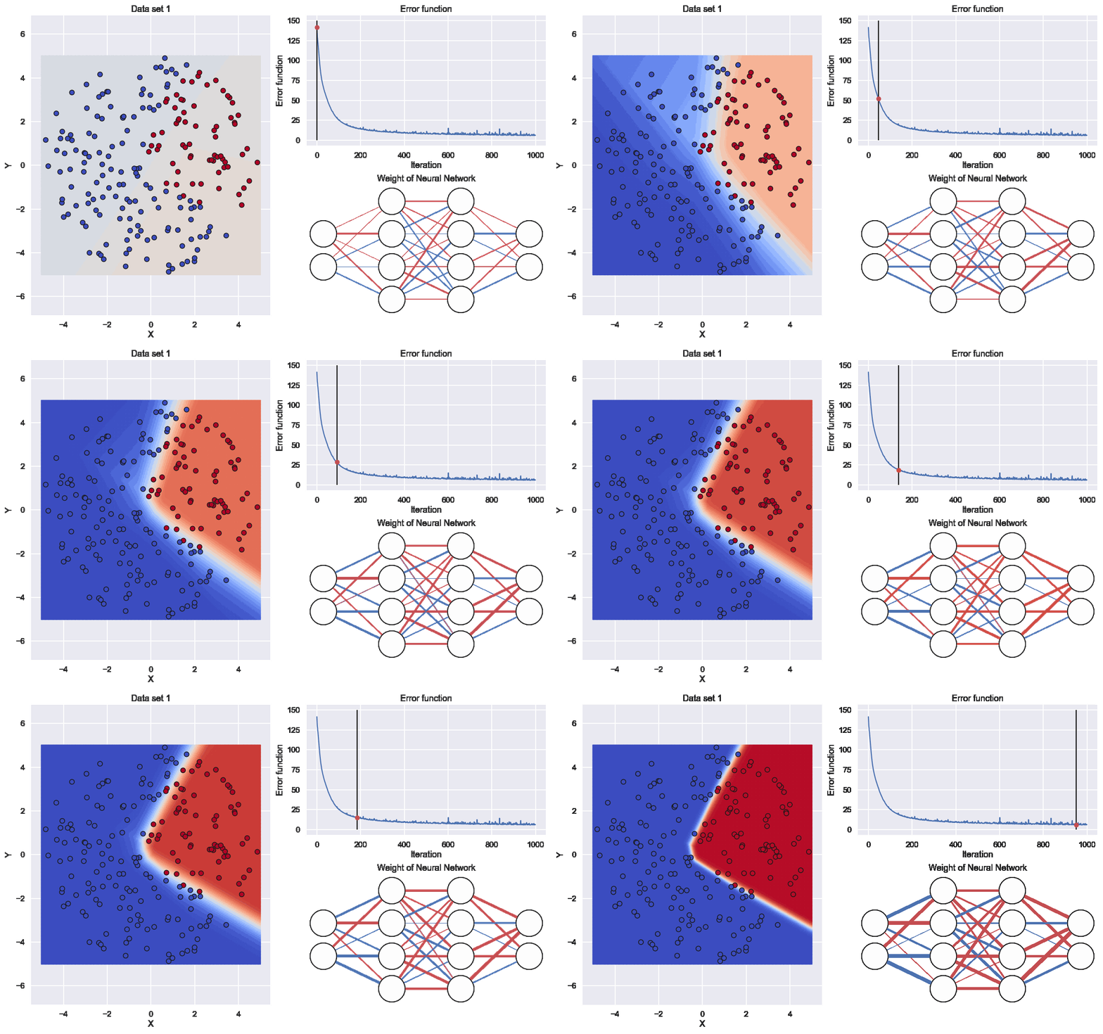
Here the graph to the lower right indicates the values of all the different weights. The thickness of the edge is related to if the (absolute)number is large or close to zero and the color resprecents if it is positive or negative
That was it! Why not just look at a different example and see who the exact same neural network would perform
One More Time
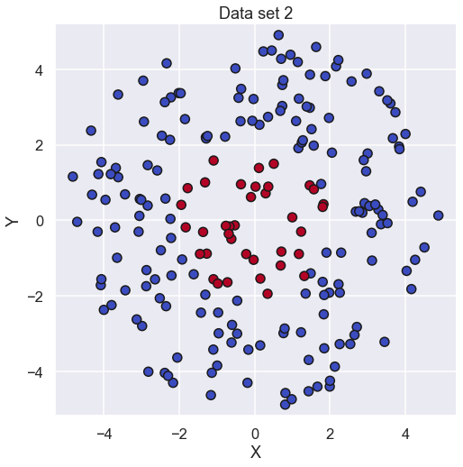
So here we have a similar data set as last time but location of the different categories are different
Now, we just run the same code as above and see what result that will come out. Starting with the value of the cost function
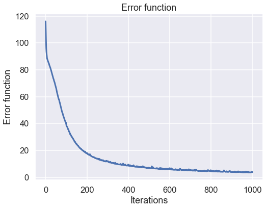
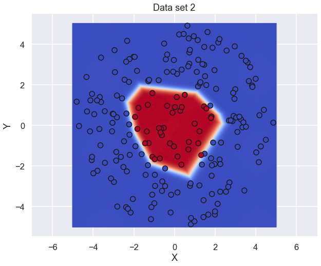
Nice, some good improvement during the training. Now for the predictions of the neural network
and, finally, an animation of the neural network during the training
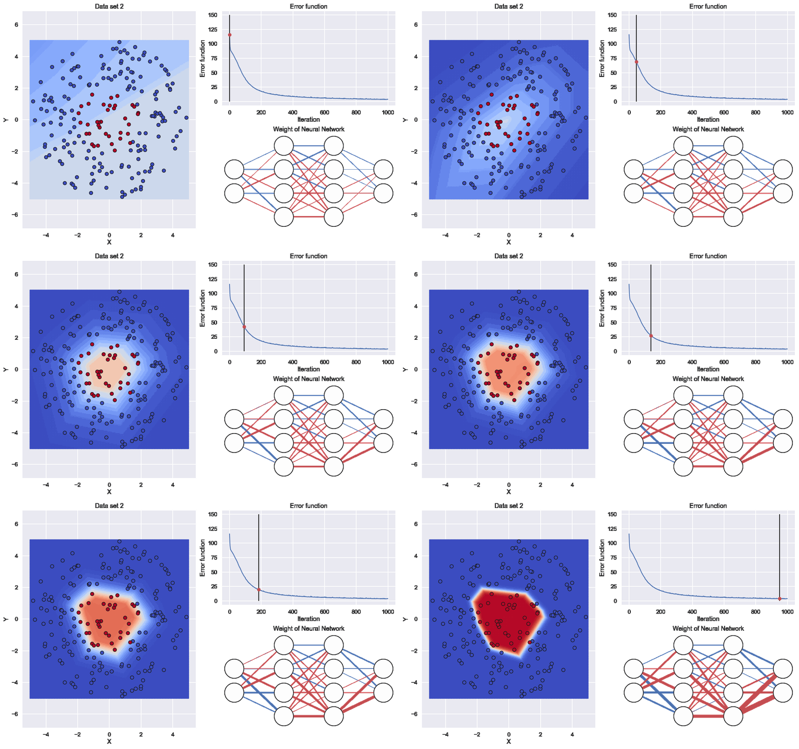
So, the exact same neural network can handle this kind of data set as well, Sweet.
Time to Conclude
Even Though this was a simple out of the box vanilla neural network the blog post was quite long... Hopefully it has shown that the concept of a neural network is quite simple and it does not require that must code to make it work. Perhaps is also has demystified the concept of "training" a neural network which seems like a strange expression.
Well I guess that was all for this time and, as always, feel free to contact us at info@gemello.se