The story of the Spectrum

In this blog post the concept of response spectrum will be discussed. The questions that we try to answer are the most basic ones: What? Why? How?

What is a Response spectrum?

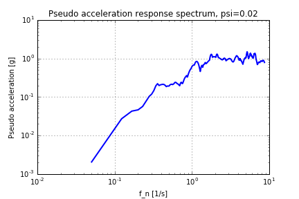
If you are working as an engineer, chances are that you might have seen a graph like the one below. The quantities that are on the axis are probably familiar, but how to use this information and how this graph is created is perhaps not obvious.

So the first question: What is a response spectrum? One, rather geeky way to explain this could be:

A Response Spectrum is a frequency based function that is used to indicate the magnitude of vibration due to a shock or transient event. A Response Spectrum can quantify transient vibration from a myriad of different events: from earthquakes to pyrotechnic events to ballistic shocks.

So, that is the What and to some extent Why. Now, let's concentrate on How such a spectrum is created and what input is needed. Imagine that some vibration or shock event is observed and somehow the time history for the acceleration can be recorded. One example of such an events is an earthquake and the time history could look something like this:

The data comes from from El Centro, California, and was recorded in the earthquake from 18 May 1940.

Now, let's imagine a house standing on the ground. This house is not a big mansion as can be found in Hollywood, but just a simple beam and mass (and some dampening). So, let’s try to expose this “house” to the time history and see what happens. Below a time history of the deformation of the “house” can be seen.

All right, not to bad (if you wonder how this graph was created just keep on reading). It can be seen that the highest deformation occurs at approximately 2.5 seconds. Let us write down that deformation value and save it for later. And when we are at it, let's also write down the properties of the “house”, that is the mass, stiffness and damping. Now, we change the properties of the house slightly and repeat the process. In this case the time history of the deformation looks like this:

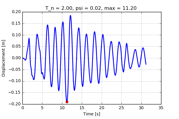
Here the maximum value can be found at 11.2 seconds. Let's record the same data as before. Having the properties of the house, it is possible to calculate the corresponding natural frequency and, after the procedure above is repeated for a lot of different natural frequencies, a plot like this can be constructed:

Sweet! There you have it, the Response Spectrum. Of course there is a bit more to it, should you record the maximum/minimum or the absolute value of the deformation? It the maximum deformation occurring within the pulse time or after? But for now, we are happy with the results. However, in the graph the quantity on the y-axis is deformation but in the first picture in this post there is acceleration. They are related by a not so complicated formula as shown below (here D is the deformation and T_n is the period time)

One relevant question is then: when you have the response spectrum, is it possible to go back to the original signal? The answer to this question is “no” unless you are extremely lucky. It is not hard to imagine, that when you only record the maximum value of the acceleration, information gets lost. For this reason, it exists infinite possibility to construct a time history that will give the same response spectrum.

OK, one more thing before we conclude: Given a time history (in this case from the earthquake) of acceleration, how is the response calculated for the beam and mass system? First some equations are needed, so let's get to it. For a single degree of freedom system, like the “building” containing a beam and mass, the equation of motion can be written as (with no external forces):

Now, let's introduce the relative displacement u_r, this is the difference between the displacement of the mass and the ground. Plugging this quantity into the equation above will result in something really cool:

Nice! What is cool is that term appearing on the right hand side is the time history of the acceleration, what is usually recorded.

The equation can be solved by a pure numerical time stepping, but there may be better ways of doing it. As the acceleration is given as a number of points in time, then it is natural to assume that the acceleration has a linear variation in time between those points. Below some python code can be found that uses this technique. More details on this can be found in reference given below.

def GetMaxResponce(k,m,psi,Dt,p):
    # Python code to compute response for 
    # SDF system given a time history of acceleration.
    # Implementation follows "Methods based of interpolation of excitation"
    # from the textbook "Dynamics of structures", A.K Chopra (second edition), 
    # chapter 5
    #
    # INPUT
    # k:         Stiffness of SDF
    # m:         Mass of SDF
    # psi:       Damping ratio
    # Dt:        Step size for time history of acceleration
    # p:         Time history of acceleration
    #
    # OUTPUT
    # t_vec:     Vector of points in time where responce are evaluated     
    # u_vec:     Deformation for times given in t_vec
    # u_dot_vec: Velocity for times given in t_vec
    
    
    omega_n = np.sqrt(k/m)
    e_omega_psi_dt = np.e**(-psi*omega_n*Dt)
    omega_d = omega_n*np.sqrt(1.0-psi**2.0)
    sin = np.sin(omega_d*Dt)
    cos = np.cos(omega_d*Dt)
    
    AA = e_omega_psi_dt * ( psi/(np.sqrt(1.0-psi**2.0))*sin + cos )
    BB = e_omega_psi_dt * (1.0/omega_d*sin)
    CC1 = ( (1.0-2.0*psi**2.0)/(omega_d*Dt) - psi/(np.sqrt(1.0-psi**2.0)) )*sin - (1.0+2.0*psi/(omega_n*Dt))*cos
    CC = 1.0/k*( 2.0*psi/(omega_n*Dt) + e_omega_psi_dt*CC1 )
    DD1 = ((2.0*psi**2.0-1.0)/(omega_d*Dt))*sin + (2.0*psi/(omega_n*Dt))*cos
    DD = (1.0-2.0*psi/(omega_n*Dt) + e_omega_psi_dt*DD1 )*1.0/k

    AAp = -e_omega_psi_dt*(omega_n/(np.sqrt(1.0-psi**2.0))*sin )
    BBp = e_omega_psi_dt*(cos - psi/(np.sqrt(1.0-psi**2.0))*sin )
    CCp1 = ( omega_n/(np.sqrt(1.0-psi**2)) + psi/(np.sqrt(1.0-psi**2)*Dt)  )*sin + 1/Dt*cos
    CCp = (-1.0/Dt + e_omega_psi_dt*CCp1)/k
    DDp1 = psi/(np.sqrt(1.0-psi**2))*sin + cos
    DDp = 1.0/(k*Dt)*(1-e_omega_psi_dt*DDp1)
    
    u, u_dot,t = 0.0, 0.0, 0.0
    t_vec = []
    u_vec = []
    u_dot_vec = []
    
    for i in range(len(p)-1):
        t_vec.append(t)
        u_vec.append(u)
        u_dot_vec.append(u_dot)
        ui = AA*u + BB*u_dot + CC*p[i] + DD*p[i+1]
        ui_dot = AAp*u + BBp*u_dot + CCp*p[i] + DDp*p[i+1]
        u = ui
        u_dot = ui_dot
        t += Dt
        
    return t_vec,u_vec,u_dot_vec

Time to conclude

In this post we have investigated what is a response spectrum and how is it constructed. However, reason why and how the spectrum is used has not been touched upon in any great detail. So, in an not so distant future, some examples related to the question Why will appear on this blog, stay tuned!

Hope you enjoyed this post and as usual, if you have questions or comments please contact us.

Reference

A.K. Chopra (2000). Dynamics of structures (Second edition). Prentice Hall